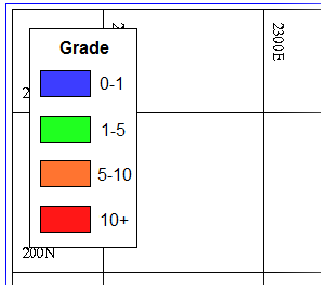
Creating a plot showing an image of a legend
In file-based plotting you can add image entities to a plot, either in the foreground so that the images appear on top of all the data except the title block, or in the background so that the images appear underneath all the data. The following task is an example of plotting with an image entity in the foreground.
Task: Creating a plot showing an image of a legend
 Note: To do this task, you need the SECTION VIEW map and the associated entities. To install this map and these entities, import entity.txt and map.txt as described earlier in this tutorial.
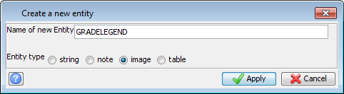
- Choose Plotting > Entity > New.
- Fill in the Create a new entity form as shown, and click Apply.
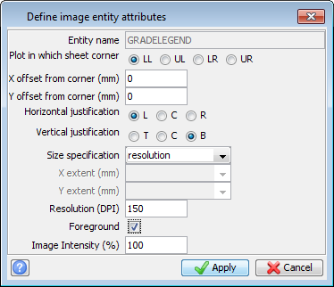
- Fill in the Define image entity attributes form as shown, and click Apply.
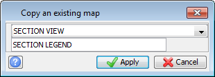
- Choose Plotting > Map > Copy.
- Fill in the form as shown, and click Apply.
- Choose Plotting > Map > Edit.
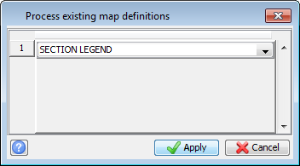
- Select SECTION LEGEND from the drop-down list, and click Apply.
- Scroll to the end of the form, right-click in the left column, and choose Add to add a new row.
- Add the GRADELEGEND entity, and set Location to grade.png — an image file of a legend that is part of the Plotting data set.
- For rows 8 to 11, and 13 to 16, in the Entity cell, type /HT1 at the end of the cell.
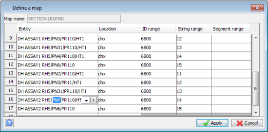
- For rows 10 and 15, in the Entity cell, change /PN4 to /PN31. Pen number 31 is an orange colour.
- For rows 11 and 16, in the Entity cell, change /PN5 to /PN4, which is red.
- Click Apply.
- Choose Plotting > Process > Map.
- Select SECTION LEGEND, and click Apply.
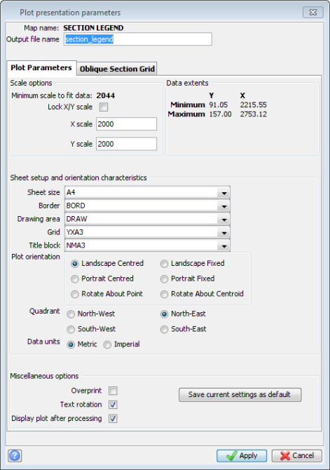
- Fill in the Plot presentation parameters form as shown, and click Apply.
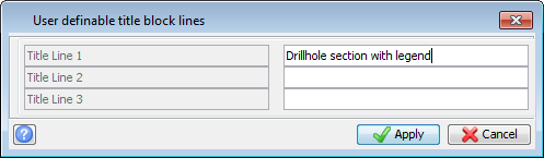
- Type some text to appear in the title block, and click Apply.
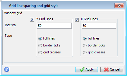
- Set the grid intervals to 50, and click Apply.
- The drillhole section, with an image legend, is created and displayed in the Plotting window.
- Choose Edit > Move plot item.
- Drag the legend to a different area of the plot, such as the upper left corner.
The SECTION VIEW map is already set up to show some drillholes. In this task, you will create a similar map that adds an image of a legend and modifies the display of the drillhole grades.
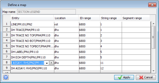
The Define a map form lists each entity in the map. This map contains several string entities, most of which are individual strings within the dhx6800.str string file. For example, line 8 of the map shows that string 11 within string file dhx6800.str will be plotted using entity DH ASSAY1 RHS to define how the string is formatted. The switch /PN2 specifies that the string is displayed using pen number 2, overriding the settings of entity DH ASSAY1 RHS. The switch /PR110 specifies that the priority of this string is 110.
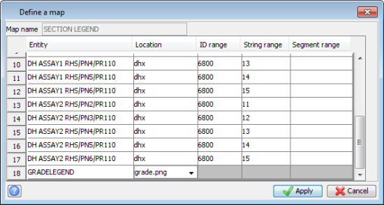
The map is set to display assay values in blue, green, red, or magenta (pen numbers 2, 3, 4, and 5 respectively) depending on the grade. Grades from 0-1 are blue, 1-5 are green, 5-10 are red, and grades above 10 are magenta. Next, you will change some of these colours, and also add a switch to reduce the text size of the assay values.
 Tip: To see the colour for each pen number, run PLOT EDIT PEN FILE, which is the menu command Plotting > Plotting colours > Pen colour properties.
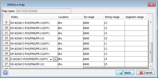
The smaller the HT number, the smaller the text. You can enter decimal numbers such as 0.8 if you want.
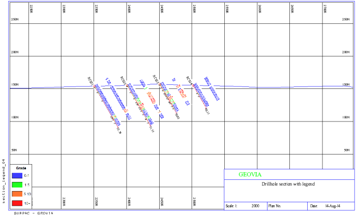
If you decide you want to adjust the location of the image after the plot is created, you can move it like any other plot item.
Tip: You can place an image above a title bock using Move plot item.