


Classify blocks
Task: Classify blocks into ore and waste
- Open blockmodel.mdl.
- Choose Column processing > Column tops.
- Enter the information as shown, and click Apply.
- Enter the information as shown, and click Apply.
- Choose Column processing > Column tops.
- Enter the information as shown, and click Apply.
- Enter the information as shown below, and click Apply.
- Choose Surfaces > DTM File functions > Create DTM from string file.
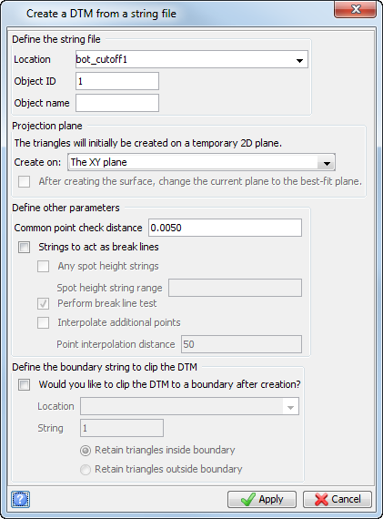
- Enter the information as shown, and click Apply.
- Choose Surfaces > DTM File functions > Create DTM from string file.
- Enter the information as shown, and click Apply.
- Choose Block model > Display.
- Enter the information as shown, and click Apply.
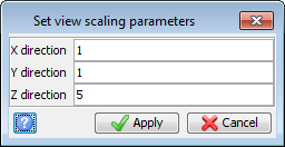
- Choose View > Data view options > View scale factors.
- Enter the information as shown, and click Apply.
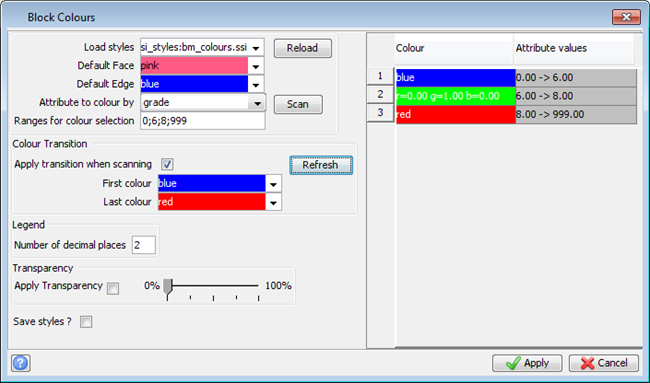
- Choose Display > Colour model by attribute.
- Enter the information as shown, click Refresh, and then click Apply.
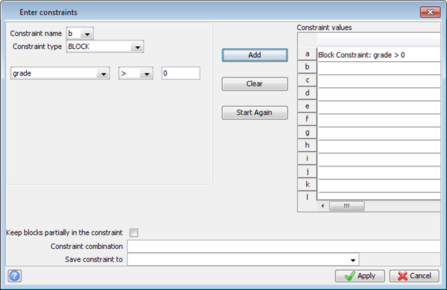
- Choose Display > New graphical constraint.
- Enter the information as shown, and click Apply.
- Open top_cutoff1.dtm and bot_cutoff1.dtm.
- Click the blockmodel button on the Status bar, and select Hide.
- Click the blockmodel button on the Status bar, and choose Display.
- Enter the information as shown, and click Apply.
- In the Layers pane, make bot_cutoff1.dtm the active layer.
- Right-click the bot_cutoff1.dtm layer and clear the Visible option.
- Make the top_cutoff1.dtm layer invisible.
- Choose Attributes > New.
- Enter the information as shown, and click Apply.
- Choose Column processing > Ore/Waste discrimination.
- Enter the information as shown, and click Apply.
- Enter the information as shown, and click Apply.
- Choose Constraints > New graphical constraint.
- Enter the information as shown, and click Apply.
- Choose Display > Colour model by attribute.
- Select ore_waste_flag for Attribute to colour by, and then click Scan.
- Click the down arrow on row 1 to bring up the Colour chooser.
- Click the Crayola tab, type in blue, and click OK.
- Click the down arrow on row 2 to display the Colour chooser.
- Click the Crayola tab, type in yellow, and click OK.
- Click Apply on the Block Colours form.
- Click Toggle display polygon & triangle edges
 to turn edges off.
 - Choose Display > View attributes for one block and click on a block.
- Choose Constraints > New graphical constraint.
- Enter the information as shown, and click Apply.
- Choose Block model > Save.
- Choose Block model > Close.
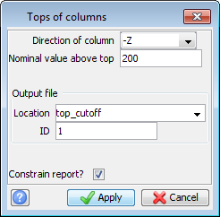
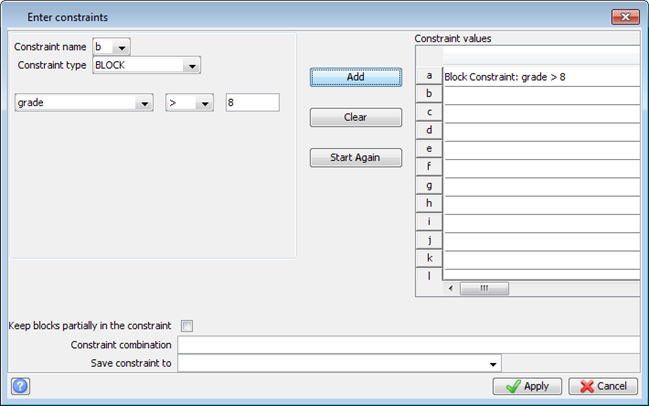
This will search down through the block model extracting a point at the top of the first block in each column where the grade is greater than 8.
The result will be a string file called top_cutoff1.str. The Nominal value above top value from the Tops of columns form is the default elevation which will be assigned if no blocks in the column satisfy the constraint. As a general rule, when extracting upper surfaces, the nominal z elevation should be set to an elevation below your model and when extracting lower surfaces it should be set to an elevation above your model.
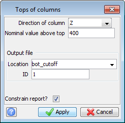
This time the search is in the Z direction (positive Z is up), and the nominal elevation is set to 400.
You will now use the string files top_cutoff1.str and bot_cutoff1.str to create DTMs.
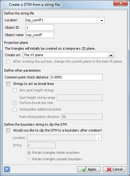
A report is displayed.
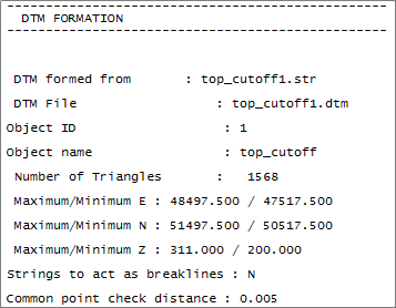
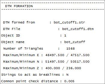
The report for the formation of this DTM is displayed.
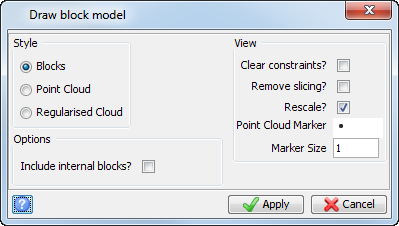
The block model with top and bottom cutoffs is displayed.
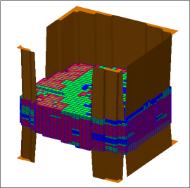
Only the upper and lower cutoff DTM surfaces are displayed.
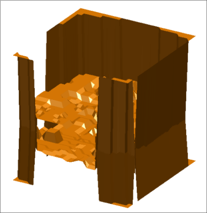
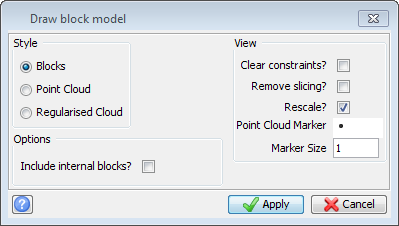
The block model is redisplayed.
The visibility icon changes from  to
to  to show that the layer is no longer visible in Graphics.
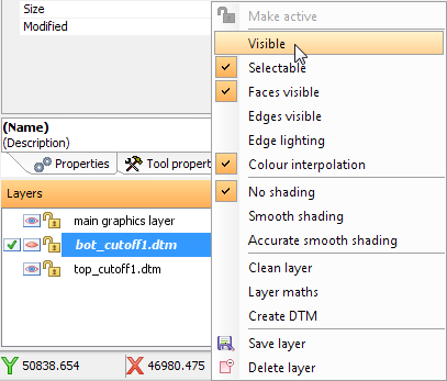
Only the block model is now visible.
The next step is to add two attributes to the model which will be filled in the Ore/Waste discrimination function.
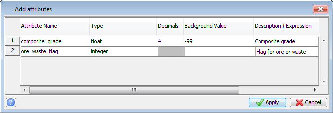
 Note: Right-click on the number 1 to add a row to the table.
The ore_waste_flag is a flag which will signify an ore block if set to 1, and a waste block if set to 0. The composite_grade attribute will store the grade for a contiguous set of ore and waste blocks in a column.
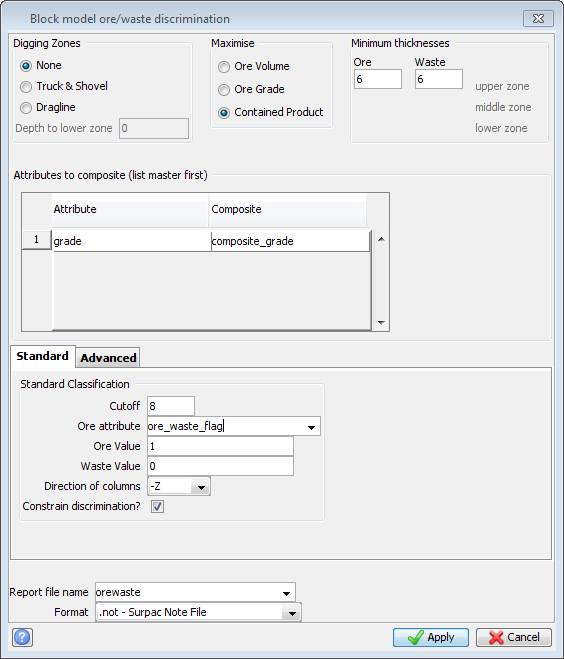
Note: You are specifying minimum mining thicknesses of ore, a waste of 6 metres, and a cutoff grade of 8.
This function classifies blocks as ORE or WASTE according to a cutoff grade and minimum thickness criteria.
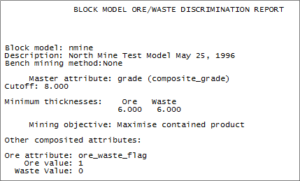
The ore/waste classification is stored as an integer value in the ore_waste_flag attribute, which allows you to colour the model on ore/waste. A master attribute is specified (grade), and an attribute to store the composite grade for each resulting ore and waste layer.
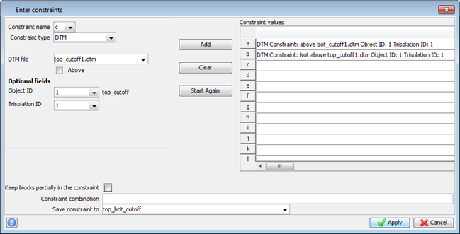
Note: It is very important that you apply this function using these two constraints. This way, no outlying sub-grade waste blocks will be included in the top or bottom ore layers. This constraint file is saved for future processing.
A summary is shown below.
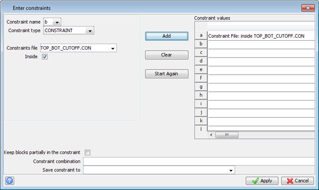
You will now colour the model on the ore_waste_flag attribute. Ensure you are viewing only the blocks within your new constraint file - top_bot_cutoff.con.
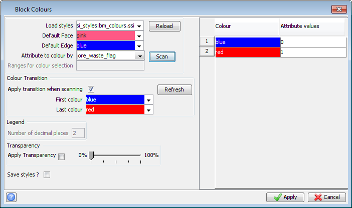
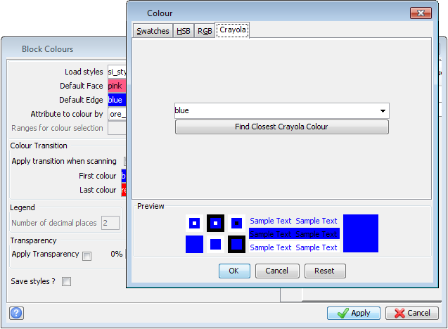
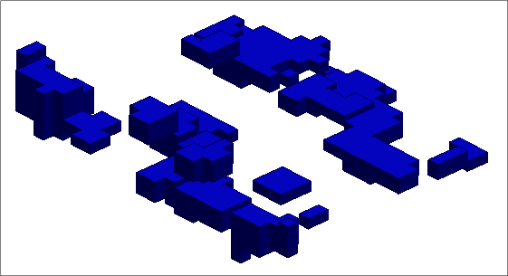
The waste blocks are now coloured blue.
The ore blocks are now coloured yellow.
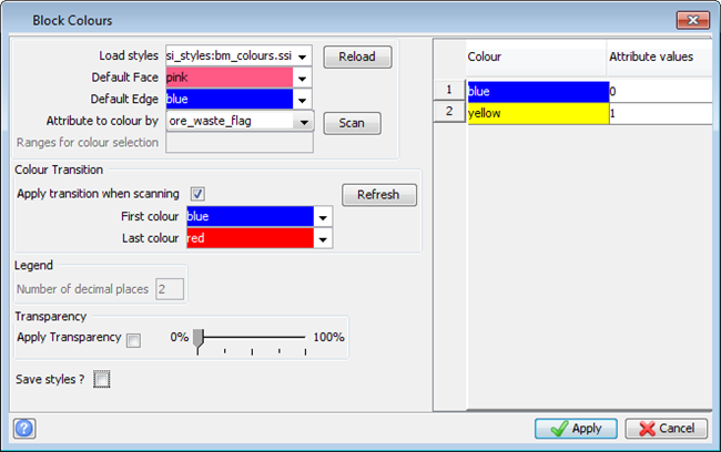
This will colour the model as shown:
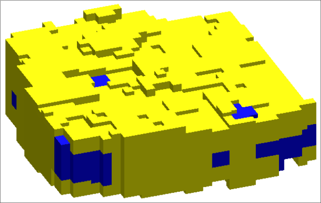
The minimum mining thickness of 6 metres (2 blocks in elevation) has been taken into account.
The composite grade is reported. This is the average grade for all contiguous ore or waste blocks in that column. If you select a block above or below this block in the same layer, it will have the same composite grade. All ore layers have a composite grade greater than 8 and all waste layers have a composite grade less than 8. You will now display waste blocks only so you can see their distribution in the model.
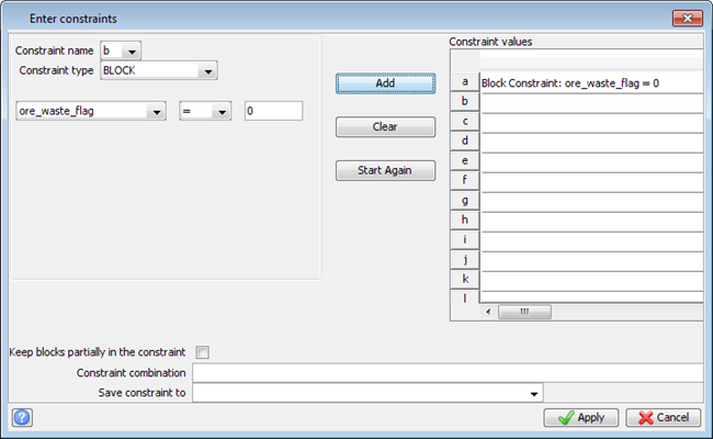
The waste blocks are displayed.
Note: To see all of the steps performed in this task, run
_11_classify_blocks.tcl.
You need to click Apply on any forms presented.