


Viewing and saving data
Multiple viewports
You can view data in different ways using multiple viewports.
Task: Work with multiple viewports
- Click Reset graphics
 .
. - Open pit_design1.str in Graphics.
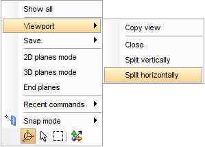
- Right-click in Graphics to display the shortcut menu.
- From the shortcut menu, select Viewport, and choose Copy view.
- Right-click the View 2 tab, and choose Close .
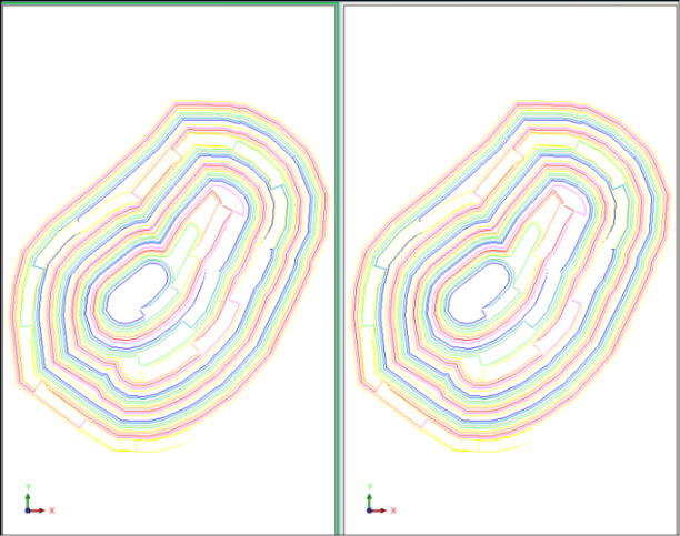
- Right-click in Graphics, and choose Viewport > Split vertically.
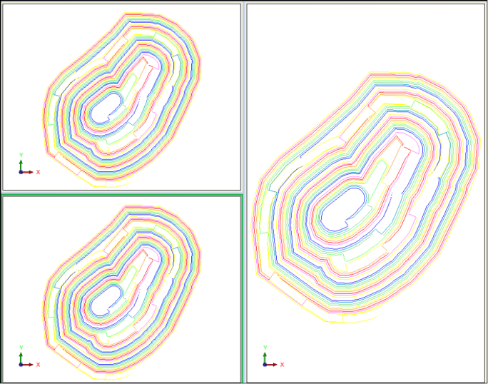
- Right-click the left viewport, and choose Viewport > Split horizontally.
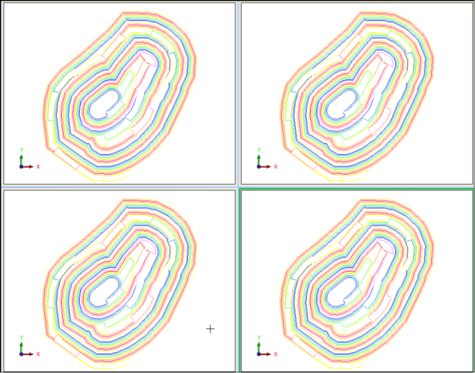
- Right-click the right viewport, and choose Viewport > Split horizontally.
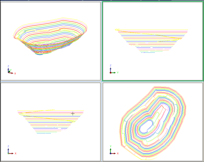
- Click and drag in the upper left viewport to rotate the data.
- Click in the lower left viewport.
- Click the
 icon to view the data in the XZ plane.
 - Click in the top right viewport.
- Click the
 icon to view the data in the YZ plane.
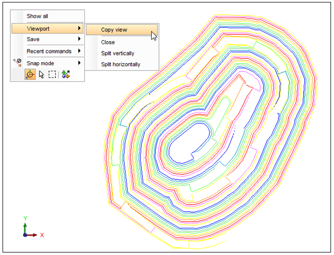
A maximised copy of the current view on a tab called View 2 is displayed.
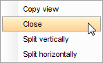
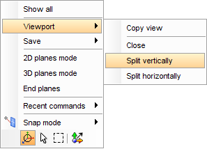
Each viewport now displays the same view of the same data.
The left viewport is split horizontally as displayed.
Four viewports are now displayed.
The data is shown in an oblique view.
Four viewports with different views of the data are displayed.
Attributes and styles files
Styles files control how strings, digital terrain models and solid models (DTM files) are displayed. You can change them to suit your needs. With styles files, you can specify many attributes, such as line colour, marker size, and drawing method (lines, markers, attributes, values).
Every time you save a string file, the associated styles file is also saved so that when the string file is next opened, it will automatically use the correct styles.
Task: Change display style
The dataset in this task represents a soil sampling study that measured arsenic concentrations at various locations. In this task you will change the display style for the points to make it easier to see where the concentrations of arsenic are highest.
- Open samp_classified1.str in Graphics.
- Click the Legend tab to show the Legend pane.
- In the Legend pane, click on the "+" sign next to Strings under the file samp_classified.str.
- In the Legend, double-click string 1.
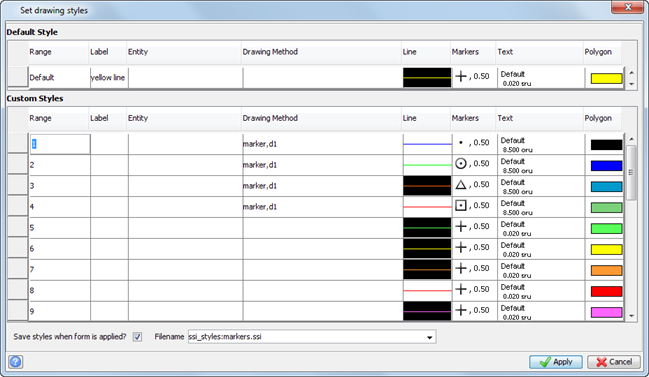
- Enter the information as shown to select the drawing method, colour, marker type, and text properties for displaying the four spot height strings.
- Type marker,d1 in the Drawing Method cell.
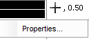
- Select the line colour by clicking the line in the line cell and selecting Properties.
- Click Edit.
- Select the colour — blue, green, orange and red for each of the four rows respectively.
- Click OK to finish the colour selection.
- Click the Markers cell, select Properties and then select the marker type.
- Click in the Text cell, select Properties, and enter oru for the Units and 8.5 for the size.
- Click Apply.
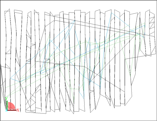
This file contains a series of points that show the concentration of arsenic in the soil. The default style settings showing the strings as coloured lines is displayed. Representing the data in this way does not help you to see where the arsenic concentration is high or low.
The points have been classified into four levels of concentration, each represented by a separate string.
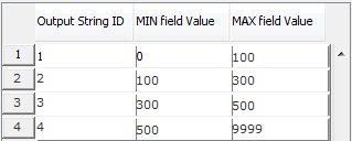
A point with an arsenic concentration of 350 parts per million (ppm), for example, forms part of string 3.
In this task, you will display the strings as spot heights to show the areas that have the highest concentration of arsenic.
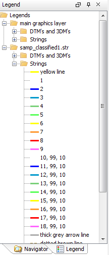
The legend shows that string 1 is white, string 2 is blue, string 3 is blue-green, and string 4 is green.
The Set Drawing Styles form is displayed.
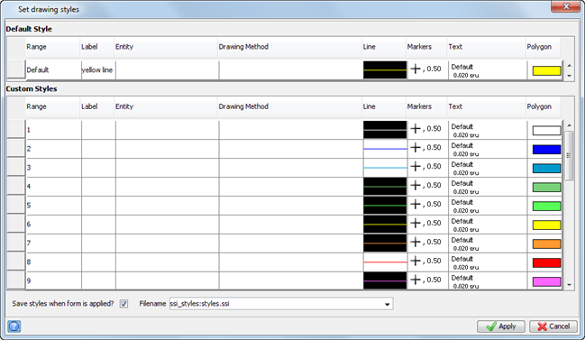
Specifically, do the following steps for each of the Custom Styles rows 1 to 4:
 Note: marker,d1 instructs Surpac to draw a marker for each point, using the d1 field as a label.
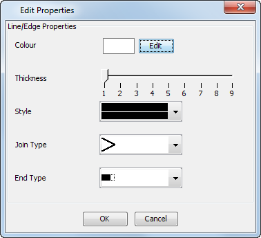
Note: You can use any of the four colour tabs shown below to select the colour of the markers and the d1 field labels.
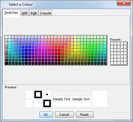
| This tab… | allows you to choose a colour by … |
|---|---|
|
Swatches |
clicking in a box on the display. |
|
HSB |
specifying its Hue, Saturation, and Brightness. |
|
RGB |
specifying its Red, Green, and Blue values |
|
Crayola |
selecting the name of the colour from a standard list of colour names. |
| For this row… | Select this marker type… |
|---|---|
|
1 |
|
|
2 |
|
|
3 |
|
|
4 |
|


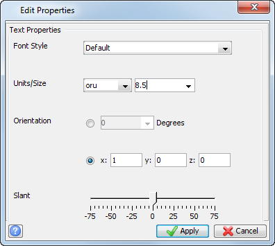
With object relative units (oru), the size of the text is set to the same units as the object. In our example, the text size for range 1 is set to 8.5 oru. The text size will be equivalent to an object that is 8.5 metres high and so will appear larger when you zoom in and smaller when you zoom out.
Note: For more information on choosing text sizes, see the
Online help.
- Click the check box in the lower left part of the form, and in the Filename box, type ssi_styles:marker.ssi.
- Click Apply.
- Zoom in and you will see numbers and symbols displayed.
- Click the Save icon on the toolbar
 .
. - Click Apply in the Save File form.

The styles are now stored in the file marker.ssi in the styles directory.
If you double click a string in the Legend pane, the Set Drawing Styles form will now look like the following.
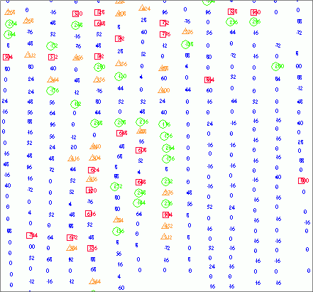
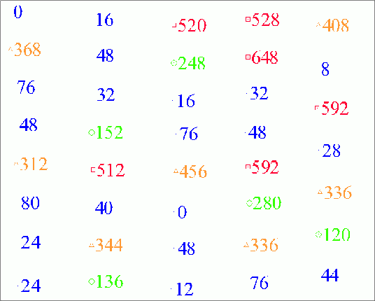
A sample of the points is displayed below. By looking at the colours, you can quickly see the areas of lowest arsenic concentration (blue), intermediate concentration (green and orange) and highest concentration (red).
The file samp_classified1.str is associated with the styles file marker.ssi. This means that when samp_classified1.str is next opened, this styles file will also load. In this way it is possible to have a collection of styles files suitable for a range of display purposes.
Note: If you want to see all of the steps
performed in this task, run 02a_change_display_styles.tcl. You
need to click Apply on
any forms presented.
Task: View point properties
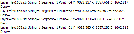
The Point properties function displays point attribute information including string, segment, and point numbers, y, x, z coordinates, and description fields.
- Click the Reset graphics icon .
- Open lev1665.str in Graphics.
- Right-click in the area next to the menu titles and select Toolbars.
- Select the Tools toolbar.
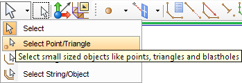
- On the Select tool drop-down, choose Select Point/Triangle.
- Hold the CTRL key and click to select any four points.
- Choose Inquire > Point properties.
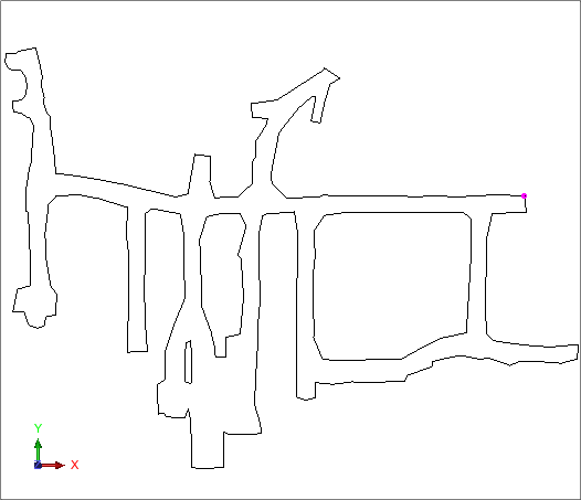
The message window displays the point properties for all of the selected points.
Note: If you want to see all of the steps
performed in this task, run 02b_view_point_properties.tcl. You
need to click Apply on
any forms presented.
Task: View segment properties
- Click Reset graphics.
- Open lev1665.str in Graphics.
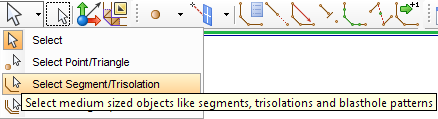
- On the Select tool drop-down, choose Select Segment/Trisolation.
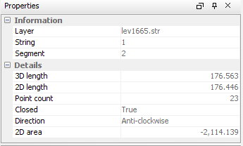
- Select the segment as shown.
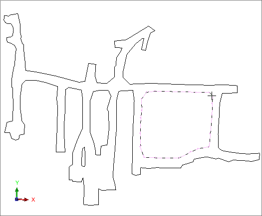
The segment properties are displayed in the Properties pane.
Note: If you want to see all of the steps
performed in this task, run 02c_view_segment_properties.tcl. You
need to click Apply on
any forms presented.
Task: Determine bearing and distance between two points
- Click Reset graphics.
- Open lev1665.str in Graphics.
- Choose Inquire > Bearing and distance between 2 points.
- Click the setup point.
- Click the foresight point.
- Press ESC to exit the fuction.
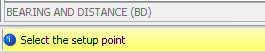
A prompt to select the setup point is displayed.
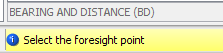
A prompt to select the foresight point is displayed.
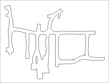
The message window displays the bearing, distance and gradient between the two points in the order in which they were selected.

Note:
To see all of the steps
performed in this task, run 02d_bearing_and_distance.tcl. You
need to click Apply on
any forms presented.
Saving data
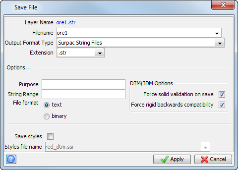
In most cases you will save strings as text files. However, if the text string files are very large (more than 5 MB), it may be worth saving them as binary files to reduce the time it takes to load the data into Graphics.
Typically, you can expect a saving of up to 15% in the size of the string file and up to 30% in the time to load the data into Graphics.
Task: Save a file
- Click Reset graphics .
- Open lev1665.str in Graphics.
- On the Select tool drop-down, choose Select Point/Triangle.
- Click on a point in Graphics.
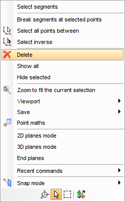
- Right-click and select Delete from the shortcut menu.
- Choose File > Save > string/DTM.
- Enter the information as shown, and click Apply.
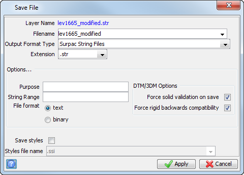
The Save function saves the contents of the active layer to a file.
 Tip: An alternative method to show the
Save File form is to click the icon
Tip: An alternative method to show the
Save File form is to click the icon  in the toolbar.
Note: To see all of the steps
performed in this task, run 02e_saving_data.tcl. You
need to click Apply on
any forms presented.