


Variogram maps
Overview
An important aspect of performing any geostatistical evaluation is to understand the anisotropy of the data, or which direction has the longest continuity. it is also important to understand how data values change with regard to the direction of longest continuity, as well as the two mutually perpendicular directions.
A variogram map is a tool within Surpac, which allows you to visualise anisotropy in a plane. Additionally, you can use variogram maps to define the anisotropy ellipsoid. These concepts are explained through the following:
- primary variogram map
- secondary variogram map
- calculation of anisotropy ellipsoid parameters
Requirements
In order to understand this information, you should:
- be familiar with Surpac string files
- know how to calculate and model a variogram in Surpac
- understand the concept of an anisotropy ellipsoid
- understand the parameters which define an anisotropy ellipsoid
Task: View variogram map dip plane
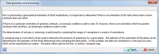
- Run 05_data_geometry.tcl.
- After reading the text on the first form, click Apply.
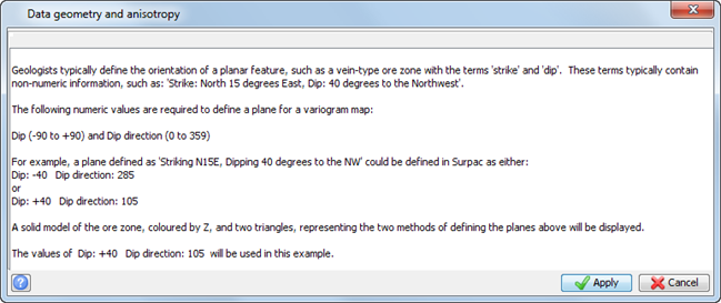
- After reading the text on the second form, click Apply.
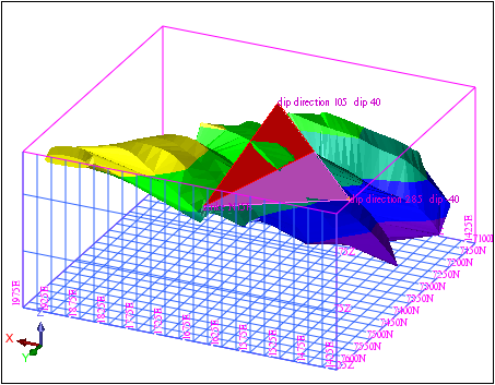
The data is displayed in Graphics.
Task: Calculate the primary variogram map
- Run 06_primary_variogram_map.tcl.
- a variogram map displayed in three dimensions
- a form displayed
- After you have viewed the primary variogram map, move the form back into view and click Apply.
- Click the Advanced tab.
- After viewing the form, click Apply.
- Read the text on the second form, then click Apply.
- Click the tab to display the orientation as shown.
You will see:
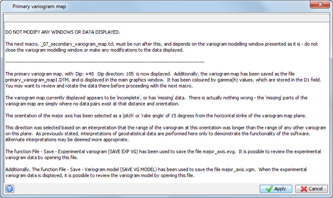
After reading the text the Primary variogram map form, move the form to the side so that you can see the image in Graphics.
 Caution: Do NOT click Apply yet.
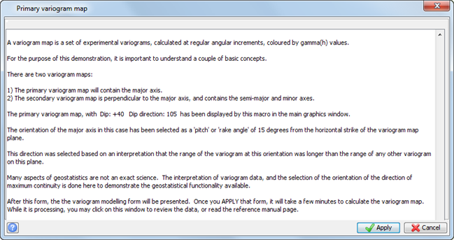
The primary variogram is displayed in Graphics.
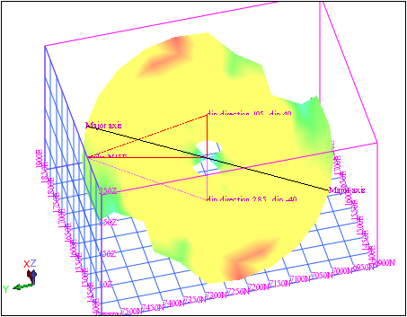
By definition, the primary variogram map will contain the major axis of the anisotropy ellipsoid. The semi-major axis could lie within the plane of the primary variogram map, but it does not have to be located on this plane.
The macro now opens the Variogram modelling window by choosing Geostatistics > Variogram modelling. It then displays the Variogram map calculation form by choosing Variogram map > New variogram map.

In the top panel, string file information (Location, ID, string range) is defined using the same parameters as in variogram calculation.
In the middle panel, the plane containing the primary variogram map is defined. You are using: Dip: +40 and Dip direction: 105.
This same plane could be defined using a dip of -40 and a dip direction of 285.
The number of variograms selected will determine the angular increment. In our example, 24 variograms will result in a 15 degree angular increment (360/24=15). If the number of variograms was set to 36, you would get a 10 degree increment (360/36=10).
The spread and spread limit parameters are the same as in normal variogram modelling.
The relationship between the angular increment and the spread angle should be considered.
It could be considered unreasonable to define a spread tolerance anything greater than half of the angular increment. For this data set, because of the small number of pairs, if a 7.5 degree spread were used (half of the 15 degree angular increment between adjacent variograms), the number of data pairs would be so small that very few, if any reasonable variograms would result. A spread of 30 degrees is used for this data set to ensure that enough samples are included to produce meaningful variograms.
Given that a spread of 30 degrees is used, you could argue that the number of variograms should be reduced to minimise the “overlap” of the cones for adjacent variograms. Although this is a reasonable argument, the resulting variograms would not be suitable to use to use to visually determine anisotropy
It is up to you, based on the data set you are working with,to determine the values you will use to produce a usable variogram without over-smoothing your data. This is an example of how geostatistics is an inexact science. Experience with a data set will usually allow you to determine what combination of parameters will give an acceptable result.
In the bottom panel, the lag, maximum distance, and variogram report parameters are specified, exactly as they are in variogram modelling. One thing you should consider is that the maximum distance will be the radius of the variogram map. You might find that you need to try a few variations of this value to get one that gives an adequate result.
You will see that the fields here are identical to those on the Advanced tab of the variogram calculation form.

You will see the variogram map, as well as the variogram for the orientation displayed on the variogram map.
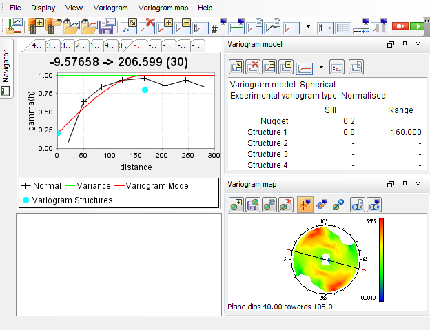
The purpose of the primary variogram map is to determine the orientation of the major axis. As described previously, by definition, the major axis lies within the primary variogram map. The example given here is based upon the premise that you, as a geologist know that the orientation of the major axis will lie somewhere in this dipping plane for this dataset. For a horizontal seam deposit, the orientation of the primary variogram map would be horizontal.
Task: Select the variogram orientation for the longest range of a given sill value
The idea is to select the variogram orientation which has the longest range for a given sill value. The lag slider can help you:
- Use the lag slider to alert you to areas of high and low variance on the variogram map. In other words, move the lag slider back and forth, and watch the colours on the variogram map change.
- Once you have an idea of what may appear to be the orientation of the longest range, click the tab for that orientation so that the black line on the variogram matches that direction.
- Now use the lag slider to improve the quality of the experimental variogram for that direction.
- After you have an acceptable variogram, create a variogram model for that orientation.
- If another orientation appears to have a longer range and a lower variance, modify the model to fit that experimental variogram. Modifying the lag distance for that orientation may help you get a better fit.
- Repeat the previous two steps until you are satisfied that you have the orientation of the major axis.
- After you have ascertained a major axis, ask yourself and others who are familiar with the geology if the orientation appears correct.
- Choose Variogram map > Select direction of maximum continuity.
- In the variogram map viewport, click and drag the red line to your selected orientation, then release.
- Click Apply to enter the value.
- Choose File > Save > Experimental variogram and model to save both the variogram and the variogram model.
You will most likely see that throughout a range of lag values, there will be areas on the variogram map which will be consistently high, and others which will be consistently low. Using the example given above, note that the orientation of 15 degrees above the horizontal (on the left) will consistently display colours on the low end of the variance values, as represented by the legend to the right.
The major axis should be that variogram which has the lowest variance for the longest distance.
As you can see, not only is the subject of variogram modelling a non-scientific process, but the orientation of the major axis is also open to interpretation and debate.
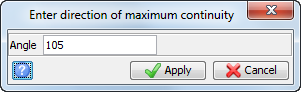
After you have determined the orientation of the major axis, you must inform the software of your selection.
A form is displayed, indicating the relative orientation of your selection, as a value between 0 and 180. You will probably need to change this value to fit your desired orientation.
 Note: This is a free rotation, and you are not forced to select a precise orientation of any of the variogram directions. This can be useful if you have found two adjacent orientations which are equally valid – you can set the direction of maximum continuity to midway between these two directions.
Task: Calculate the secondary variogram map
- Run 07_secondary_variogram_map.tcl.
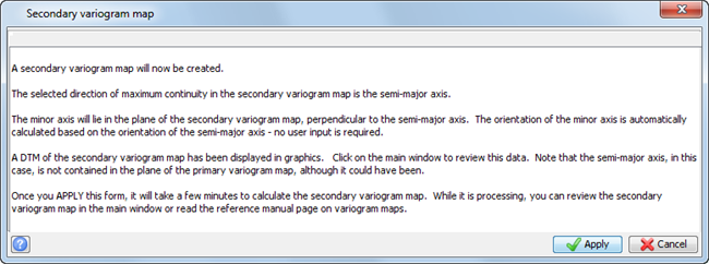
- After reading the text on the following form, click Apply.
- After reading the text on the following form, click Apply.
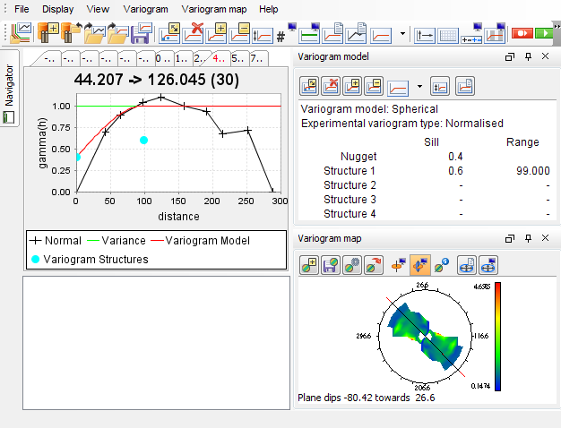
- Click the tab to display the orientation as shown.
Note: If you want to know the steps to perform this task manually see Task: Use the Secondary Variogram Map to Define the Semi-Major Axis at the end of this topic.
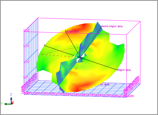
The secondary variogram map, and the selected orientations of all axes, are displayed in Graphics.
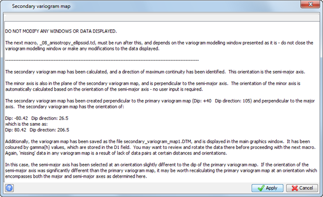
Note: The same steps used to select the direction of maximum continuity for the primary variogram map have been used to select the direction of maximum continuity for the secondary variogram map.
Anisotropy ellipsoid parameters
Task: Calculate ellipsoid parameters with a macro
- Run 08_anisotropy_ellipsoid.tcl.
- After reading the text on the first form, click Apply.
- After reading the text on the following form, click Apply.
- After reading the text on the following form, click Apply.
- When the next form is displayed, click and drag it out of the way so that you can view the variogram modelled for the minor axis.
- After reading the text on the following form, click Apply.
- After reading the text on the following form, click Apply.
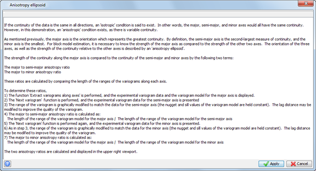
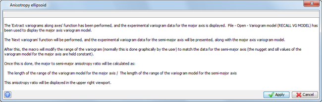
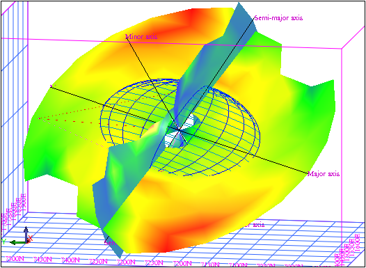
The secondary variogram map, and the selected orientations of all axes are displayed.
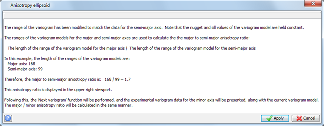
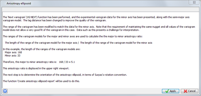
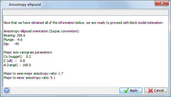
You will see the ellipsoid displayed in Graphics.
Task: Calculate ellipsoid parameters manually
- Choose Variogram map > Secondary variogram map.
- Choose Variogram map > Extract variograms along axes.
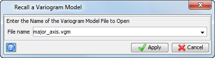
- Choose File > Open > Variogram model.
- Enter the information as shown, and click Apply.
- Click the semi-major tab.
- Click and drag the variogram structure to the left, until the model matches the experimental variogram, as shown.
- Click the minor tab.
- Click and drag the variogram structure to the left, until the model matches the experimental variogram, as shown.
- Choose Variogram Map > Create anisotropy ellipsoid report.
- Enter the information as shown, and click Apply.
- If the file exists, the Confirm File Replace form appears. Click Yes.
- Choose Variogram Map > Ellipsoid visualiser.
- Enter the information as shown, and click Save Now.
- Click Apply.
- In the main Surpac main window, choose Display > Hide grid.
- Open ellipsoid123.str in Graphics.
- In the Variogram modelling window, choose File > Close.
The variogram model is displayed.


Note: The major/semi-major anisotropy ratio changes as you move the model.

Note: The major/semi-major anisotropy ratio changes as you move the model.


It should resemble the previous ellipsoid created by the macro.

Steps for using variogram maps to create anisotropy ellipsoid parameters
In summary, here are the complete set of steps to obtain all of the anisotropy ellipsoid parameters:
Task: Use the primary variogram map to define the major axis
- Choose Geostatistics > Variogram modelling to open the Variogram modelling window.
- Choose Variogram map > New variogram map.
- Enter the variogram map parameters and click Apply.
- Use the lag slider to show you areas of high and low variance on the variogram map. That is, move the lag slider back and forth, and watch the colours on the variogram map change. You will most likely see that throughout a range of lag values, there will be areas on the variogram map which will be consistently high, and others which will be consistently low. Using the example given above, note that the orientation of 15 degrees above the horizontal (on the left) will consistently display colours on the low end of the variance values, as represented by the legend to the right, and that very small lag values are usually not useful.
- Once you have an idea of what appears to be the orientation of the longest range, select the variogram tab that represents that orientation.
- Use the lag slider to improve the quality of the experimental variogram for that direction.
- Create a variogram model for that orientation.
- Look at the model on all other orientations. The major axis should be that variogram which has the lowest variance for the longest distance.
- If another orientation appears to have a longer range and a lower variance than your current model, modify the model to fit that experimental variogram.
- Repeat the previous two steps until you are satisfied that you have the orientation of the major axis. Choose File > Save > Variogram model to save a variogram (*.vgm) for this orientation. Saving this is optional, but can be helpful in a future step.
- Choose Variogram map > Select direction of maximum continuity.
- Click and drag the red line on the variogram map until it is aligned with the orientation of the major axis.
- Choose Variogram map > Save DTM. This is an optional step, but can help you to display the orientation of the primary variogram map in three dimensions in Graphics.
Task: Use the secondary variogram map to Ddfine the semi-major axis
- Choose Variogram map > Secondary Variogram map. The direction of maximum continuity (the red line) will display as the intersection of the primary and secondary variogram maps. The orientation of this line should be relatively close to what will become the semi-major axis.
- Select a variogram to rotate the black line on the variogram map to that direction.
- Now use the lag slider to improve the quality of the experimental variogram for that direction.
- Create a variogram model for this orientation, which will become the semi-major axis. You can choose Display > Display/Hide variance to show the data variance (often used as the total sill).
- Look at the model on all other orientations. The semi-major axis should be that variogram which has the lowest variance for the longest distance.
- If another orientation appears to have a longer range and a lower variance than your current model, modify the model to fit that experimental variogram.
- Repeat the previous two steps until you are satisfied that you have the orientation of the semi-major axis.
- Choose Variogram map > Select direction of maximum continuity.
- Click and drag the red line on the variogram map until it is aligned with the orientation of maximum continuity.
- Choose Variogram map > Save DTM. This is an optional step, but can help you to display the orientation of the secondary variogram map in three dimensions in Graphics.
Task: Create and view anisotropy ellipsoid parameters
- Choose Variogram map> Extract variograms along axes.
- Choose File> Open > Variogram model to display the variogram model for the major axis. If you did not previously save a variogram model, create a variogram to fit the major axis.
- Ensure that the variogram for the semi-major axis is either the same as, or to the left of, the variogram model for the major axis. You might need to use the lag slider to improve the quality of the variogram. By definition, the range of the major axis must be equal to, or longer than, the range of the semi-major axis for a given sill.
- If the variogram representing the semi-major axis is to the right of the model for the major axis, you need to start again. The current semi-major axis is a more likely candidate for the orientation of the major axis.
- Ensure that the variogram for the minor axis is either the same as, or to the left of the variogram model for the semi-major axis. You might need to use the lag slider to improve the quality of the variogram. By definition, the range of the semi-major axis must be equal to, or longer than, the range of the minor axis for a given sill.
- If the variogram representing the minor axis is to the right of the model for the semi-major axis, you need to go back to the secondary variogram map. The current minor axis is a more likely candidate for the orientation of the semi-major axis.
- View the semi-major axis. Modify the lag if required to improve the quality of the experimental variogram.
- Click and drag the sill/range marker to the left until the variogram model matches the experimental variogram for the semi-major axis.
- View the minor axis. Modify the lag if required to improve the quality of the experimental variogram.
- Click and drag the sill/range marker to the left until the variogram model matches the experimental variogram for the minor axis.
- Choose Variogram map > Create anisotropy ellipsoid report. This report contains values for the orientation of the anisotropy ellipsoid, as well as the major/semi-major and major/minor anisotropy ratios.
- Choose Variogram map > Ellipsoid visualiser. You can view or save the ellipsoid.
- Choose File > Close to exit the Variogram modelling window.
Note: It is often difficult or impossible to interpret the experimental variogram for the minor direction. If you cannot get a visually acceptable minor variogram, but you do have good quality variograms for the major and semi-major axes, you can choose to continue. Then you can determine the ratio for the minor axis based on other factors, such as geometry.
Note: You will not be able to modify either the nugget or the sill - only the range is changed to calculate the anisotropy ratio.
Note: It is often difficult or impossible to interpret the experimental variogram for the minor direction. If you cannot get a visually acceptable minor variogram, but you do have good quality variograms for the major and semi-major axes, you can choose to modify the range until the ratio for the minor axis is equal to some value you have chosen based on other factors, such as geometry.