


Calculating an experimental variogram
Overview
An experimental variogram is calculated from pairs of data points, which can be limited to points that are aligned in a specific orientation (directional), or without limiting them to an orientation (omnidirectional). The experimental variogram is used as the basis for creating a variogram model. In order to create a variogram model, the experimental variogram must appear relatively smooth. Adjusting the lag distance can help to create a smooth variogram. If the data contains outliers, or a small number of data points, the experimental variogram can appear jagged, or "noisy". It often takes several iterations and combinations of parameters to create experimental variograms that are acceptable for modelling.
You will learn about:
- calculating omnidirectional and directional variograms
- changing the display
- saving a variogram
Requirements
In order to understand this information, you should:
- be familiar with Surpac string files
- know how to run a Surpac macro
- understand basic variogram concepts, such as nugget, sill, and lag
- understand the difference between omnidirectional and directional variograms
Task: Create and view experimental variograms
This you will calculate omnidirectional and directional variograms from the D1 field of the file gc_zone1_cut130.str.
- Choose Geostatistics > Variogram modelling.
- Choose File > New > String file variogram.
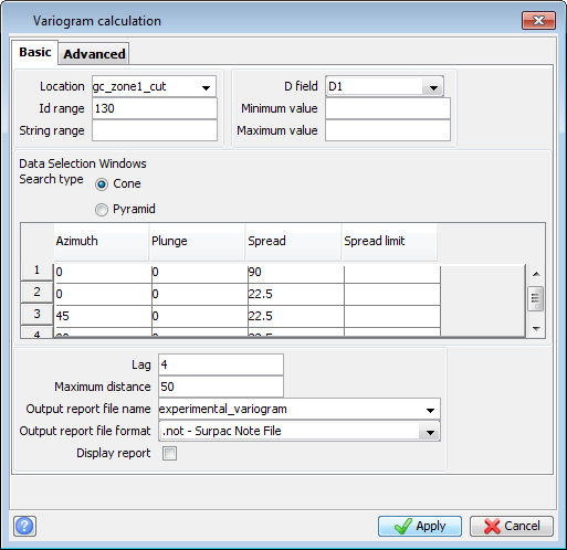
- On the Basic tab, enter the information as shown.
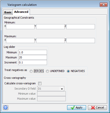
- On the Advanced tab, enter the information as shown, and click Apply.
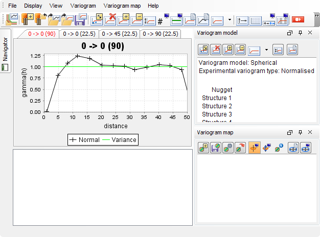
- Click each tab to display the variogram for that orientation.
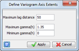
- Choose Display > Set axis limits.
- Enter the information as shown, and click Apply.
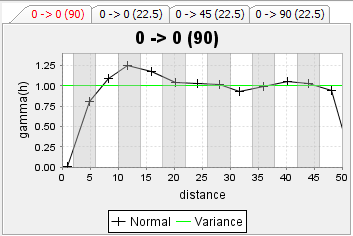
- Choose Display > Display / Hide lag intervals.
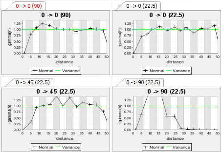
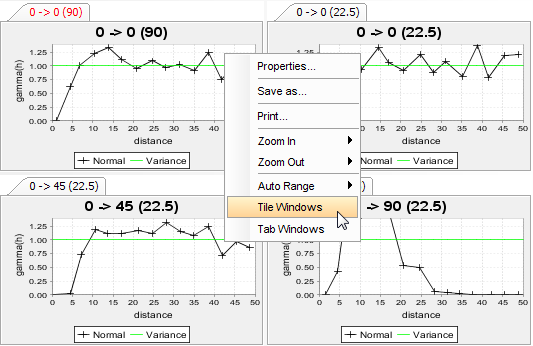
- Right click anywhere on the variogram window, and then select Tile Windows.
- Change the lag by:
- clicking and dragging the lag slider.
- clicking the lag increment/decrement arrows on either side of the lag slider.
- pressing the right arrow or left arrow keys on the keyboard.
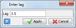
- Choose Variogram > Experimental variogram lag.
- Enter the information as shown, and click Apply.
- Choose Display > Display / Hide lag intervals to remove the lag intervals.
- Right click anywhere on any variogram chart, and select Tab Windows.
- Select the tab labelled 0 -> 0 (90).
- Select Display > All orientations chart
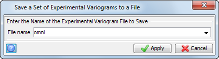
- Choose File > Save > Experimental variogram.
- Enter the information as shown, and click Apply.
- Choose File > Close to exit the variogram modelling window.
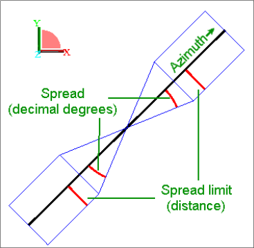
 Note: To
calculate an omnidirectional variogram, set the Spread
to 90.
Note: To
calculate an omnidirectional variogram, set the Spread
to 90.
The omnidirectional variogram will appear on the first of four tabs.
The lag intervals appear.
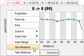
All variograms will appear tiled.
As you do any of the above, the variogram shape and the lag intervals will change.
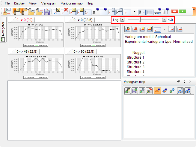
Note: Changing the lag is one of the most common ways to attempt to get a "good looking" variogram.
The omnidirectional variogram is displayed.
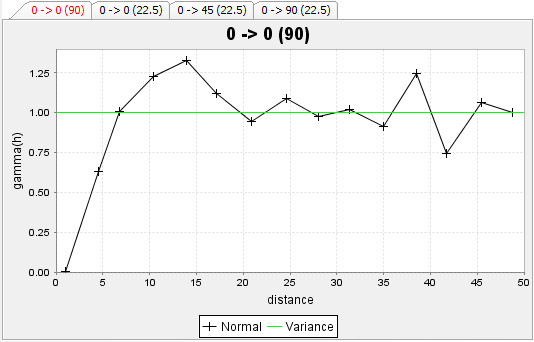
All experimental variograms are displayed together.
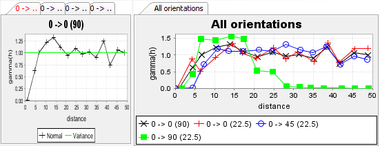
Note: To see all of the steps performed in this task. run 2d_05a_experimental_variogram.tcl. You need to click Apply on any forms presented.
Types of experimental variograms
Once an experimental variogram has been calculated, it can be transformed by several different methods.
Task: Change the variogram type
- Open omni.evg.
- Choose Variogram > Type.
- Select Standard, and click Apply.
- Choose Variogram > Type.
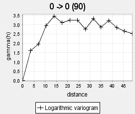
- Select Logarithmic, and click Apply.
- Choose Variogram > Type.
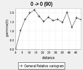
- Select General Relative, and click Apply.
- Choose Variogram > Type.
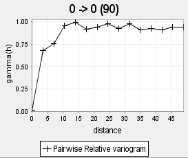
- Select Pairwise Relative, and click Apply.
The Variogram Modelling window opens, and the normalised variogram is displayed.
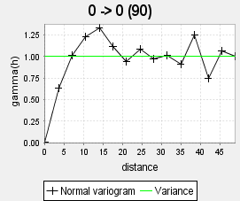
Note: Not only does the shape of the variogram change, but the gamma(h) values are also modified. If the variance of the data was displayed, it is now removed.
Note: The shape in this case is identical to the normal variogram, but the gamma (h) values are different. They have been divided by the value of the variance of the data set.
Note: The shape in this case is different to the normal and general relative, and the gamma(h) values are different.
|
|
|
|
|
|
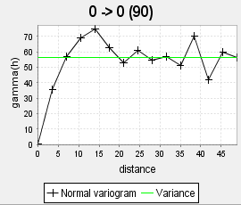
Logarithmic variogram
In this type of a variogram, logarithms of the raw data are used to calculate the experimental variogram. Any negative or zero raw data values are first set to small positive values before a logarithmic transformation is applied. If the distribution of your data is logarithmic, or near logarithmic, and a reasonable fit cannot be obtained from a normal variogram, a logarithmic variogram can potentially give a usable value which can be used for the range of a normal variogram.
General Relative variogram
In this type of a variogram, each gamma(h) is divided by the squared mean of all samples used to estimate that gamma(h).
If local values within the population are affected by the local variance, a condition called a “proportional effect” is said to exist. “Relative” variograms can be more useful than “normal” variograms if a proportional effect exists.
Pairwise Relative variogram
In this type of variogram, the squared difference of each sample pair is divided by the square of the mean of each sample pair. Similarly to the logarithmic variogram, units along the Y (gamma(h)) axis have no meaning but the relative variograms may serve to identify ranges and structures
Note: The application of these types of variograms is an advanced topic. If you wish to obtain more information on this, you should obtain instruction from a qualified geostatistical consultant.
Note: To see all of the steps performed in this task, run2d_05b_variogram_types.tcl. You need to click Apply on any forms presented.
Menu commands:
| Select... | to... |
|---|---|
| Geostatistics > Variogram modelling | open the Variogram Modelling Window. |
| From the Variogram Modelling Window: | |
| Variogram > New string file variogram | calculate one or more variograms. |
| Display > Set axis limits | set the X and Y values of the variogram graph area. |
| Display > Lag intervals | toggle the lag intervals on and off. |
| Variogram > Experimental variogram lag | set the lag exactly. |
| Variogram > Model | create a new model and allows editing (click and drag the blue dots). |
| File > Save > Experimental variogram and model | create *.EVG and *.VGM files. |