


Basic statistics
Overview
One of the important preliminary steps in performing a geostatistical evaluation is to understand the statistical properties of the data. Two characteristics which can potentially reduce the quality of your estimations are bimodalism and outliers. You can use a histogram to identify both of these.
You will learn about:
- histograms
- bimodal distributions
- creating a histogram.
Requirements
In order to understand this information, you should:
- be familiar with Surpac string files
- know how to run a Surpac macro.
Histograms
A histogram is a statistical term which refers to a graph of frequency against value. A histogram is the graphical version of a table which shows what proportion of cases fall into each of several non-overlapping intervals of some variable.
For example, you could represent a distribution of gold grades with the following table:
| Gold (g/t) |
Number of samples (frequency) |
|---|---|
| 0.0 - 0.5 | 0 |
| 0.5 – 1.0 | 40 |
| 1.0 - 1.5 | 58 |
| 1.5 – 2.0 | 82 |
| 2.0 - 2.5 | 40 |
| 2.5 – 3.0 | 29 |
| 3.0 - 3.5 | 18 |
| 3.5 – 4.0 | 10 |
| 4.0 – 4.5 | 12 |
| 4.5 – 5.0 | 5 |
| 5.5 – 6.0 | 5 |
| 6.0 – 6.5 | 5 |
| 6.5 – 7.0 | 5 |
| 7.0 – 7.5 | 8 |
| 7.5 – 8.0 | 5 |
You can display this same data in a histogram as shown:

Bimodal distributions
The "mode" is the most commonly occurring value in a data set. For example, in the following data set, the number 8 is the mode:
1 3 5 5 8 8 8 9
"Bimodal" means that there are two relatively "most common" values which are not adjacent to one another. In the following data set, the numbers 2 and 8 are equally common, and the distribution is said to be "bimodal":
1 2 2 2 3 5 5 8 8 8 9
Imagine that you are studying the average specific gravity, or density of rocks in a coal deposit. A histogram of all rock samples might look like this:
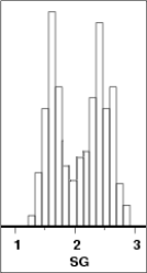
Any histogram which displays two peaks, as in the previous example, is said to be "bimodal". You can explain the bimodal distribution in the previous example by the fact that the data set is comprised of coal samples as well as intervening sandstone and mudstone bands. The specific gravity values between 1 and 2 are representative of the coal, while specific gravity values between 2 and 3 represent the intervening rock.
Often the source of a bimodal distribution can be two domains being mixed into a single data set. In order to minimise estimation errors, you should make every attempt to separate any data set which has a bimodal distribution. In the example above, simply segregating the data based on rock type would result in two separate normal distributions.
Creating a histogram
Task: Create a histogram from string data
- Choose Geostatistics > Basic statistics.
- Choose File > Load data from string files.
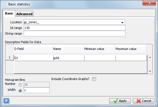
- Enter the information as shown, and click Apply:
- Choose Display > Histogram.
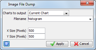
- Choose File > Save as > Image file.
- Enter the information as shown, and click Apply:
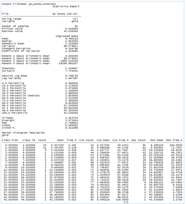
- Choose Statistics > Report.
- Enter the information as shown, and click Apply:
- Close the Basic Statistics window.
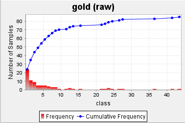
The histogram and cumulative frequency are displayed:
The histogram is displayed:
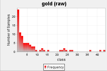
The image (as above) is saved in the current working directory.

The file gc_zone1_130stats.not is created and displayed:
To see all of the steps performed in this task run 2d_02a_basic_statistics_histogram.tcl..
 Note: The Basic Statistics Window must be closed when running the file.
Task: Create a log-probability plot from string data
- Choose Geostatistics > Basic statistics.
- Choose File > Load data from string files.
- Enter the information as shown, and click Apply:
- Choose Statistics > Transformations.
- Enter the information as shown, and click Apply:
- Choose Display > Probability Curve.
- Choose File > Save as > Image file.
- Enter the information as shown, and click Apply:
- Close the Basic Statistics window.
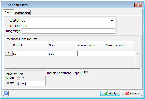
The histogram and cumulative frequency are displayed for the D1 values in gc130.str:

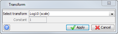
The histogram and cumulative frequency for the transformed data are displayed:

The histogram and cumulative frequency are displayed, as shown:

Note: The Log-Probability graph will be a straight line for a true lognormal distribution.
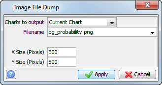
The image (as above) is saved in the current working directory.
Notes:
- To see all of the steps performed in this task run 2d_02b_basic_statistics_logprobability.tcl.
- The Basic Statistics Window must be closed.
Menu commands:
| Select... | to... |
|---|---|
| Geostatistics > Basic statistics | open the Basic Statistics window. |
| From the Statistics Window: | |
| File > Load data from string files | load the drillhole data. |
| Display > Histogram | create a histogram. |
| Statistics > Report | create a report. |
| File > Save as > Image file | save the histogram as an image. |
| Statistics > Transformations | scale the data. |
| Display > Probability Curve | create a log probability plot. |