


Anisotropy
Overview
An important aspect of performing any geostatistical evaluation is to understand how data values change with regard to direction. The term "anisotropy" explains this concept.
You will learn about:
- isotropy and anisotropy
- geostatistical estimation using isotropy
- geostatistical estimation using anisotropy
- Ellipsoid Visualiser
Requirements
In order to understand this information, you should:
- be familiar with Surpac string files, and how to display them
- be familiar with the geometric shape and deposition of economic geological deposits
- understand the concept of a centroid of an individual block in a block model
Isotropy vs. anisotropy
In order to understand anisotropy, it is helpful to know what the term isotropy refers to. Here is a definition of each term:
Isotropy: The property of being isotropic; having the same value when measured in different directions.
Anisotropy: The property of being anisotropic; having a different value when measured in different directions.
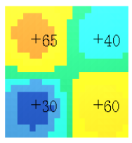
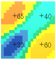
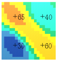
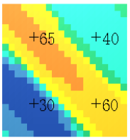
When estimating values in a block model, the amount and direction of anisotropy can have a significant impact on the end result. For example, the three models shown below were created from the same data set, but different amounts of anisotropy were used.
|
|
|
|
No Anisotropy (Isotropic) |
2:1 Anisotropy Azimuth 45 |
|
|
|
|
2:1 Anisotropy Azimuth 135 |
5:1 Anisotropy Azimuth 135 |
Task: Display block models created with anisotropy
- Run 2d_04_anisotropy.tcl
- Click in Graphics after each model is displayed.
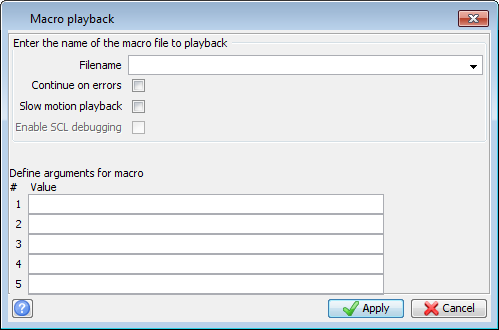
If you use the Macro playback button, you can see all values on the forms by selecting Slow motion playback:
In geostatistical terms, isotropy, or an isotropic condition, is said to exist when the rate of change of data values is the same in all directions. A true isotropic condition in three dimensions is rare for most types of data. However, an isotropic condition in two dimensions is more common. For example, the rate of change of alumina values in a large horizontal bauxite deposit beneath relatively flat topography may be isotropic in the XY plane.
Conversely, anisotropy, or an anisotropic condition is said to exist when the rate of change of data values is different in different directions. This is probably the most common case. For example, an epithermal gold vein may have different rates of change in each of any three mutually perpendicular directions: along strike, down dip, and perpendicular to the dip plane.
The remainder of this chapter will explain the use of isotropy and anisotropy in performing geostatistical estimations. To understand how you determine whether a data set is isotropic or anisotropic, and how to calculate the direction and amount of anisotropy, you will need to study the chapters on variograms and variogram maps.
Geostatistical estimation using isotropy
In geostatistical estimation (for example, inverse distance weighting, ordinary kriging, and indicator kriging), one or more points, usually representing sample locations, are used to estimate a value at a location where there are no samples. For example, in the image below, the sample locations are represented by two points in a Surpac string file. In this string file, D1 contains the sample values (D1=10 for one point, and D1=20 for the other point). The location to be estimated is the centre position, or "centroid" of a 1 x 1 x 1 block of material.
In this example, you will assume that all data is in the XY plane (that is, the sample points and the block centroid each have the same Z value). You will also assume that you are estimating a value at the block centroid (at coordinates 0N, 0E), and that only the two samples shown will be used for the estimation. Notice that both samples are the same distance (3 metres) from the block centroid. If you assume that the material surrounding the block and samples is homogenous (all the same), you can assume that there is no "directional continuity" within the data, and the two samples will contribute equally to the estimation. Another way of stating this is that the "weight" applied to both samples will be equal.
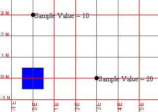
In this situation, where only two samples are used to estimate the value for the block, the "weight" for each sample will be 0.5. The calculation of the block value is:
( sample value1 * weight1 ) + ( sample value2 * weight2 ) = block value
( 10 * 0.5 ) + ( 20 * 0.5 ) = 15
Throughout this tutorial, you will assume that the sum of the weights must equal 1. In other words,
weight1 + weight2 = 0.5 + 0.5 = 1.0
When you assume that there is no directional continuity within the data, you say that you have an "isotropic" condition. In the example below, again assuming that all data is in the XY plane, any sample whose location is on the following circle will be given the same weight as any other sample on that circle during the estimation of the value of the block centroid. In two dimensions, when the shape defining the line of equal weights is a circle, you are said to be performing an "isotropic" estimation.
This means that you are assuming that the direction from the point being estimated to the sample is not important, and that only the distance from the sample to the block centroid is important.

In the previous example, because all sample locations are the same distance from the block centroid, all samples are given equal weight. The calculation of the block value is:
( 5 * 0.25 ) + ( 10 * 0.25 ) + ( 20 * 0.25 ) + ( 35 * 0.25 ) = 17.5
As mentioned before, the sum of all the weights must be equal to 1.0:
0.25 + 0.25 + 0.25 + 0.25 = 1.0
In three dimensions, during isotropic estimation, any samples falling on the surface of the same sphere are given equal weight.

In the example above, all sample locations are on the surface of the same sphere, and are thus the same distance from the block centroid. In this three-dimensional example of an isotropic condition, all samples are given equal weight. The calculation of the block value is:
( 10 * 0.333 ) + ( 20 * 0.333 ) + ( 40 * 0.333 ) = 23.333
Again, the sum of all the weights is 1.0 (assuming that 1/3 + 1/3 + 1/3 expressed as decimals equals 1):
0.333 + 0.333 + 0.333 = 0.999 = 1.0
In Surpac, when you are performing an estimation, you are prompted to fill in values defining the orientation of the "major axis" and the "anisotropy ratios". You will cover these topics later. For now, if you wish to perform an estimation assuming that the data is isotropic, use the following values:
BEARING OF MAJOR AXIS: 0 (or any value from 0 to 360)
PLUNGE OF MAJOR AXIS: 0 (or any value from -90 to 90)
DIP OF SEMI-MAJOR AXIS: 0 (or any value from -90 to 90)
MAJOR/SEMI-MAJOR ANISOTROPY RATIO: 1
MAJOR/MINOR ANISOTROPY RATIO: 1
Task: View an example of an isotropic sphere
- Open isotropic_ellipsoid1.str.
- Display the D1 values for string 1
The isotropic ellipsoid is displayed, with all axes labelled.
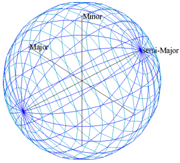
The concepts of "major axis", "semi-major axis" and "minor axis" are explained later. For now, just understand that the lengths of all of these axes are the same for an isotropic ellipsoid.
Geostatistical estimation using anisotropy
As previously stated, an anisotropic condition is said to exist when the rate of change of data values is different in different directions. This is the case for nearly all data sets which represent samples taken from the earth. Anisotropic conditions can result from geological conditions, such as fracturing or deposition method. For example, in plan view, the correlation, or similarity, of samples taken along strike in a gold-bearing quartz vein may be better than the correlation of samples taken across strike. In a sedimentary deposit, such as a flat-lying coal seam, samples may be better correlated within the horizontal plane than vertically through the seam. When a data set has anisotropy, the direction from the point being estimated to a sample location is important.
How much anisotropy is present is also important. The determination of the magnitude of anisotropy for a data set may be done qualitatively or quantitatively (by intuition or by numerical calculation). For example, after becoming familiar with a silver deposit consisting of a vertical vein trending east to west (strike: 90 degrees, dip: 90 degrees) a geologist may say that "there's about 3 times more continuity along strike (horizontally) than across strike (horizontally)". As rough and unsubstantiated a statement as this may seem, many times this type of qualitative judgement is actually used in geostatistical estimation. In this situation, you would say that there is a "3 to 1 anisotropy ratio" in the horizontal plane. This is commonly written as "a 3:1 anisotropy ratio". The direction of maximum continuity is referred to as the "major axis". In the silver vein example, the major axis could be defined as a bearing of either 90 or 270 degrees - they are both the same in geostatistical terms. In two dimensions, you can represent a 3:1 anisotropy ratio with a major axis bearing 90 degrees with an ellipse, such as shown below:
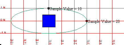
When you want to use anisotropy during an estimation, the direction from the location being estimated to the sample is important. In this example, you will assume that the point being estimated is the centroid of the block, and that you will use only two samples, as shown above, to estimate a value for the block.
Even though the sample, that has a value of 10, is 1 metre from the block centroid, and the sample that has a value of 20 is 3 metres from the block centroid, the two samples would be given the same weight in this situation. This is because "anisotropic distances" are used in the calculation of the weights, and not actual distances. Recall that you have indicated that there is a 3:1 anisotropy ratio and the bearing of the major axis is 90 degrees. Samples oriented due north or south of the block, such as the sample whose value is 10, will have their anisotropic distances calculated as the actual distance (1, in this case) multiplied by the anisotropy ratio (3, in this case). Thus, the anisotropic distance calculated for the sample whose value is 10 is:
Actual Distance x Anisotropy Ratio = Anisotropic Distance
1x3=3
This calculation is displayed in the following table for both samples:
| Sample Value | Sample Bearing | Actual Distance | Anisotropy Factor | Anisotropic Distance | Weight |
|---|---|---|---|---|---|
| 10 | 0 | 1 | 3 | 3 | 0.5 |
| 20 | 90 | 3 | 1 | 3 | 0.5 |
Because the anisotropic distances are the same, the weights for the points are the same. The calculation of the block value is:
( 10 * 0.5 ) + ( 20 * 0.5 ) = 15
If the sample whose value is 10 is moved to a position at Y=3, X=0, and you again use a 3:1 anisotropy ratio with the bearing of the major axis at 90 degrees (or 270 degrees), as shown below, the weights assigned to both samples will change.
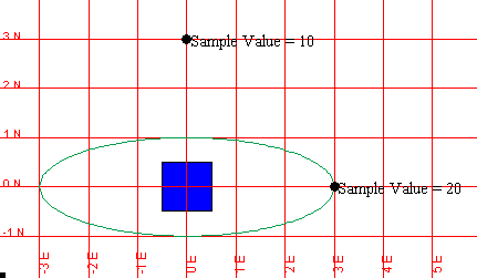
The anisotropic distance of the sample whose value is 10 is now 9: Actual Distance (3) X Anisotropy Ratio (3) = Anisotropic Distance (9). This calculation is displayed in the following table for both samples.
| Sample Value | Sample Bearing | Actual Distance | Anisotropy Factor | Anisotropic Distance | Weight |
|---|---|---|---|---|---|
| 10 | 0 | 3 | 3 | 9 | 0.25 |
| 20 | 90 | 3 | 1 | 3 | 0.75 |
The weights of the samples now change to take account of the new anisotropic distances. The calculation of the block value is now:
( 10 * 0.25 ) + ( 20 * 0.75 ) = 17.5
Notice that the calculation of the weights here is only approximate to demonstrate the effects of anisotropy. In actual practice, the geostatistical method you decide to use will affect the values of the weights.
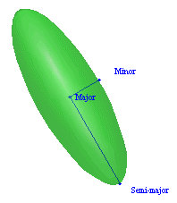
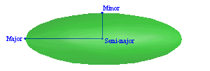
Assuming that our geologist has another opinion that "there is about 2 times more continuity horizontally along strike than vertically (up and down) within the plane of the vein", you would say that there is a "2:1 anisotropy ratio" in the vertical YZ plane. In two dimensions, an ellipse represents the line where weights are equal. In three dimensions, this shape is called an "ellipsoid". So now you have a 3:1 anisotropy ratio in the horizontal XY plane, and a 2:1 anisotropy ratio in the vertical YZ plane. You distinguish between these ratios by defining three axes for the ellipsoid:
Major axis
Semi-major axis
Minor axis
By definition, the major axis is the longest, the semi-major axis is the second longest, and the minor axis is the shortest. Also, all three axes are mutually perpendicular to one another.
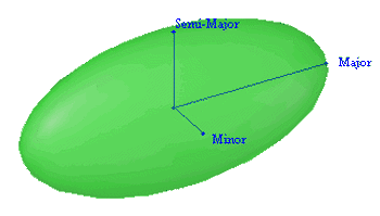
The ratio between the length of the major axis and the length of the semi-major axis is defined as the MAJOR/SEMI-MAJOR ANISOTROPY RATIO. The ratio between the length of the major axis and the length of the minor axis is defined as the MAJOR/MINOR ANISOTROPY RATIO.
When you perform an estimation, and want to use three-dimensional anisotropy, any samples falling on the surface of the same ellipsoid will be given equal weight. In the example below, all sample locations are on the surface of the same ellipsoid, and so, all the samples are all considered to be the same anisotropic distance from the block centroid:
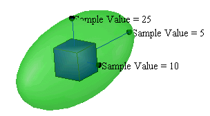
With the axes oriented as above, as well as a major/semi-major anisotropy ratio of 2, and a major/minor anisotropy ratio of 3, the calculation of the weights for the data as shown is:
| Axis | Sample Value | Sample Bearing |
Sample Dip | Actual Distance |
Anisotropy Factor |
Anisotropic Distance |
Weight |
|---|---|---|---|---|---|---|---|
| Major | 5 | 90 | 0 | 3 | 1 | 3 | 0.333 |
| Semi-Major | 25 | 0 | 90 | 1.5 | 2 | 3 | 0.333 |
| Minor | 10 | 180 | 0 | 1 | 3 | 3 | 0.333 |
Because the anisotropic distances are the same, the weights for the points are the same. The calculation of the block value is:
( 5 * 0.333 ) + ( 25 * 0.333 ) + ( 10 * 0.333 ) = 13.3333
Again, the sum of all the weights is 1.0 (assuming that 1/3 + 1/3 + 1/3 expressed as decimals equals 1):
0.333 + 0.333 + 0.333 = 0.999 = 1.0
If the distance from the block centroid to each sample is now the same, the weights will change. For example, in the view below, the distance from each sample to the block centroid is now 3, but you are still using the same anisotropy ellipsoid:
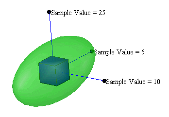
The calculation of the weights is as follows:
| Axis | Sample Value | Sample Bearing |
Sample Dip | Actual Distance |
Anisotropy Factor |
Anisotropic Distance |
Weight |
|---|---|---|---|---|---|---|---|
| Major | 5 | 90 | 0 | 3 | 1 | 3 | 0.74 |
| Semi-Major | 25 | 0 | 90 | 3 | 2 | 6 | 0.18 |
| Minor | 10 | 180 | 0 | 3 | 3 | 9 | 0.08 |
The calculation of the block value is:
( 5 * 0.74 ) + ( 25 * 0.18 ) + ( 10 * 0.08 ) = 9.0
Again, the sum of all the weights is 1.0 :
0.74 + 0.18 + 0.08 = 1.0
Ellipsoid visualiser
Using our previous example where you have a major/minor anisotropy ratio of 3, and a major/semi-major anisotropy ratio of 2, you would get an ellipsoid, but you need to establish the orientation of the ellipsoid. In Surpac, this can be accomplished in several different ways, including the "Surpac" method. The examples which follow use the "Surpac" method, which encompasses the following three terms:
| Term | Min | Max | Description |
|---|---|---|---|
| Bearing of major axis | 0 | 360 | azimuth of major axis in XY plane |
| Plunge of major axis | -90 | 90 | dip above or below horizontal plane |
| Dip of semi-major axis | -90 | 90 | rotation of semi-major axis around major axis |
The Ellipsoid Visualiser is a tool which can assist you to understand the orientation of the anisotropy ellipsoid. You will now use it to create several anisotropy ellipsoids, and save them as Surpac string files.
Task: Display anisotropy using the ellipsoid visualiser
- Choose Geostatistics > Ellipsoid visualiser.
- Enter the values of bearing, plunge, and dip.
- Click and drag the image of the ellipsoid to rotate it.
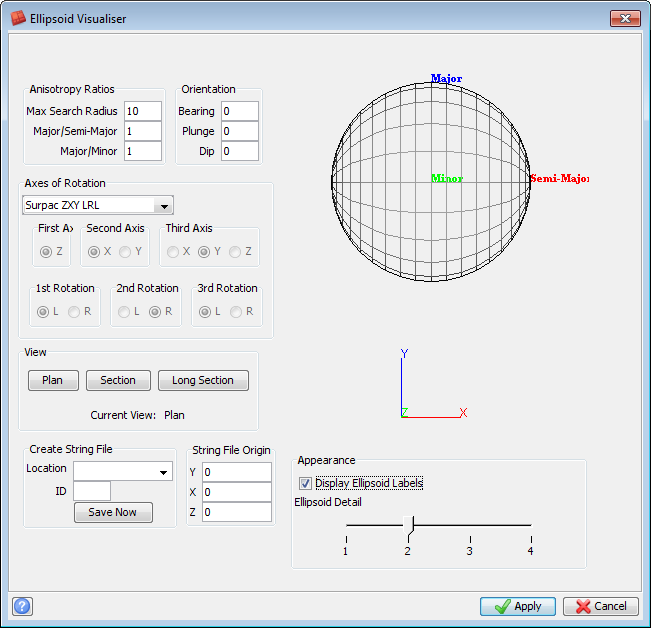
For each example below:
Example #1:
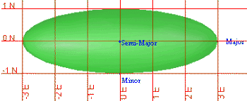
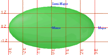
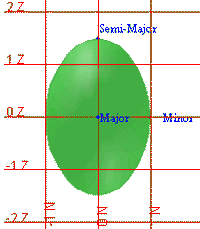
You could use this ellipsoid to estimate gold values within a vertical vein that has strike: 90 degrees and dip: 90 degrees.
| Bearing of major axis | 90 |
| Plunge of major axis | 0 |
| Dip of semi-major axis | -90 |
| Major/semi-major anisotropy ratio | 2 |
| Major/minor anisotropy ratio | 3 |
| 3D View |
Looking down on XY plane major/minor anisotropy ratio: 3 |
|
|
|
|
Looking north at XZ plane major/semi-major anisotropy ratio: 2 |
Looking west at YZ plane dip of semi-major axis: 90 |
|
|
|
Example #2:
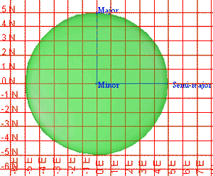
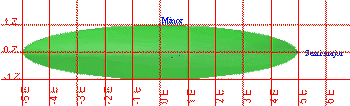
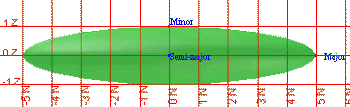
This ellipsoid could be used to estimate values within a horizontal coal seam or other data from flat-lying sedimentary rocks, where continuity within the seam is the same in the XY plane (major/semi-major anisotropy ratio: 1), but the continuity is significantly less in the vertical direction.
| Bearing of major axis | 0 |
| Plunge of major axis | 0 |
| Dip of semi-major axis | 0 |
| Major/semi-major anisotropy ratio | 1 |
| Major/minor anisotropy ratio | 5 |
| 3D View |
Looking down on XY plane major/semi-major anisotropy ratio: 1 |
|
|
|
|
Looking north at XZ plane dip of semi-major axis: 0 |
Looking west at YZ plane major/minor anisotropy ratio: 5 |
|
|
|
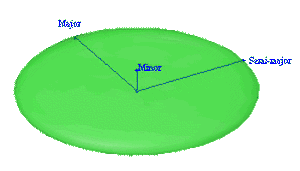
Example #3:
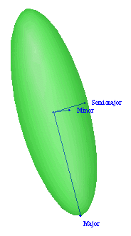
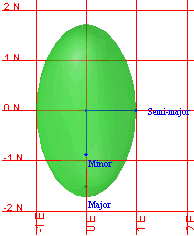
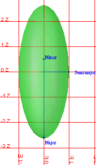
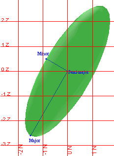
This ellipsoid could be used to estimate values from a kimberlitic diatreme, or diamond-bearing "pipe" type ore body, which plunges to the south at a dip of 60 degrees below the horizontal.
| Bearing of major axis | 180 |
| Plunge of major axis | -60 |
| Dip of semi-major axis | 0 |
| Major/semi-major anisotropy ratio | 3 |
| Major/minor anisotropy ratio | 3 |
| 3D View |
Looking down on XY plane major/semi-major anisotropy ratio: 3 |
|
|
|
|
Looking north at XZ plane dip of semi-major axis: 0 |
Looking west at YZ plane major/minor anisotropy ratio: 3 |
|
|
|
Example #4:
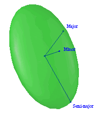
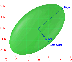
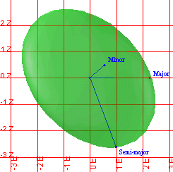
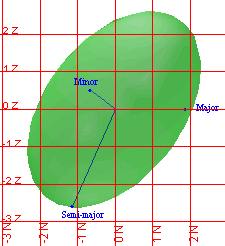
This ellipsoid could be used to estimate values from an epithermal vein, with strike of 50 degrees and dip to the southeast of 60 degrees below the horizontal, where continuity within the vein is the same in all directions (major/semi-major anisotropy ratio: 1).
| Bearing of major axis | 50 |
| Plunge of major axis | 0 |
| Dip of semi-major axis | -60 |
| Major/semi-major anisotropy ratio | 1 |
| Major/minor anisotropy ratio | 3 |
| 3D View | Looking down on XY plane |
|
|
|
| Looking north at XZ plane | Looking west at YZ plane |
|
|
|
Example #4(continued)
|
Looking horizontally along strike: az 50 degrees, dip 0 Note dip of semi-major axis is -60 degrees major/semi-major anisotropy ratio: 1 |
Looking downdip: azimuth 140 degrees, dip -60 Note major axis is along strike, semi-major is downdip major/minor anisotropy ratio: 3 |
|
|
|
Menu commands:
| Select... | to... |
|---|---|
| Geostatistics > Ellipsoid visualiser | view the ellipsoid. |