Basic Statistics
The Histogram
A histogram is a statistical term which refers to a graph of frequency vs. value. A histogram is the graphical version of a table which shows what proportion of cases fall into each of several non-overlapping intervals of some variable.
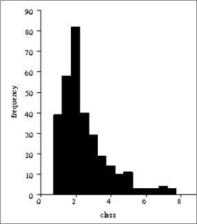
For example, you could represent a distribution of gold grades with the following table:
| Gold (g/t) |
Number of samples (frequency) |
|---|---|
| 0.0 - 0.5 | 0 |
| 0.5 – 1.0 | 40 |
| 1.0 - 1.5 | 58 |
| 1.5 – 2.0 | 82 |
| 2.0 - 2.5 | 40 |
| 2.5 – 3.0 | 29 |
| 3.0 - 3.5 | 18 |
| 3.5 – 4.0 | 10 |
| 4.0 – 4.5 | 12 |
| 4.5 – 5.0 | 5 |
| 5.5 – 6.0 | 5 |
| 6.0 – 6.5 | 5 |
| 6.5 – 7.0 | 5 |
| 7.0 – 7.5 | 8 |
| 7.5 – 8.0 | 5 |
You can display this same data in a histogram as shown:
Bimodal Distributions
The "mode" is the most commonly occurring value in a data set. For example, in the following data set, the number 8 is the mode:
1 3 5 5 8 8 8 9
"Bimodal" means that there are two relatively "most common" values which are not adjacent to one another. In the following data set, the numbers 2 and 8 are equally common, and the distribution is said to be "bimodal":
1 2 2 2 3 5 5 8 8 8 9
Imagine that you are studying the average specific gravity, or density of rocks in a coal deposit. A histogram of all rock samples might look like this:
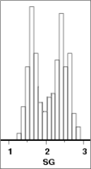
Any histogram which displays two peaks, as in the previous example, is said to be "bimodal". You can explain the bimodal distribution in the previous example by the fact that the data set is comprised of coal samples as well as intervening sandstone and mudstone bands. The specific gravity values between 1 and 2 are representative of the coal, while specific gravity values between 2 and 3 represent the intervening rock.
Often the source of a bimodal distribution can be two domains being mixed into a single data set. In order to minimise estimation errors, you should make every attempt to separate any data set which has a bimodal distribution. In the example above, merely segregating the data based on rock type would result in two separate normal distributions.
Outliers
An "outlier" is a statistical term for a value that is significantly different than the majority of all other values in the data set. For example, in the following data set, the number 236 would be considered to be an outlier:
1 3 5 5 8 8 8 236
Outliers can cause "noisy" experimental variograms, which are difficult to model. Additionally, if you use outliers in an estimation, they can cause unrealistic results. One technique to reduce the effect of outliers is to apply a "cutoff", or "topcut" to them. In the previous example, the value of 236 could be "cut", or changed to a value of 9:
1 3 5 5 8 8 8 9
Another alternative is to remove the outlier values.
Displaying Histograms in Surpac
Task: Display Histogram
- Run the macro 08a_basic_statistics.tcl.
- After reading the text below on the first form, click Apply.
- After reviewing the form, click Apply.
- When you have finished viewing the form, click Apply.
- After reading the text displayed on the next form, click Apply.
|
Basic statistics should be performed before variogram modelling for a couple of reasons:
1. The shape of the histogram can be used to determine if a distribution is bimodal (has two humps). If the histogram shows a bimodal distribution, the data should be analysed graphically to see if it can be physically segregated into two separate zones. If so, each zone should be modelled separately.
2. The quality of experimental variograms and subsequent block model estimations are sensitive to outliers (relatively large values).
Outlier values should be cut or removed prior to variogram modelling or block model estimation. The value used to cut or remove outliers can be calculated from information in the basic statistics report. |
The macro runs Analysis > Basic statistics window to open the Basic Statistics window.
The macro then runs File > Load data from string files.
The following form is displayed.
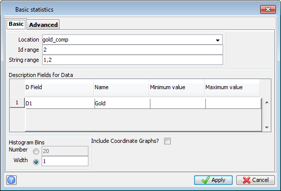
Basic Statistics on gold_comp2.str
You will use strings 1 and 2 from the file gold_comp2.str as the basis of your study. The columns labelled "Minimum value" and "Maximum value" allow you to exclude data which is below a given minimum value or above a given maximum value.
On the Advanced tab, you can exclude data which is greater or less than any Y, X, or Z coordinate values.
The D1 field contains values of gold in grams per tonne. The Name field is optional. The name value will appear on the output report.
Also, note that it is possible to view the histogram based on a number of bins or on a bin width. The "bin width" method is more commonly used.
Next, a histogram and a line representing the cumulative frequency is displayed. The cumulative frequency is an accumulation of the values of all previous histogram bins.
The macro then runs Statistics > Report. This form prompts you to enter the name of an output report, the report format, and a range of percentiles which will be written to the report.
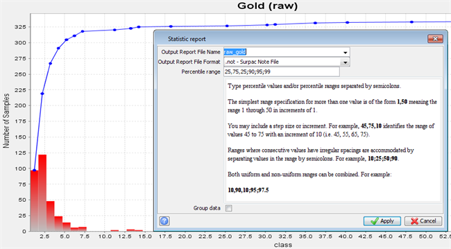
Basic statistics histogram and report
|
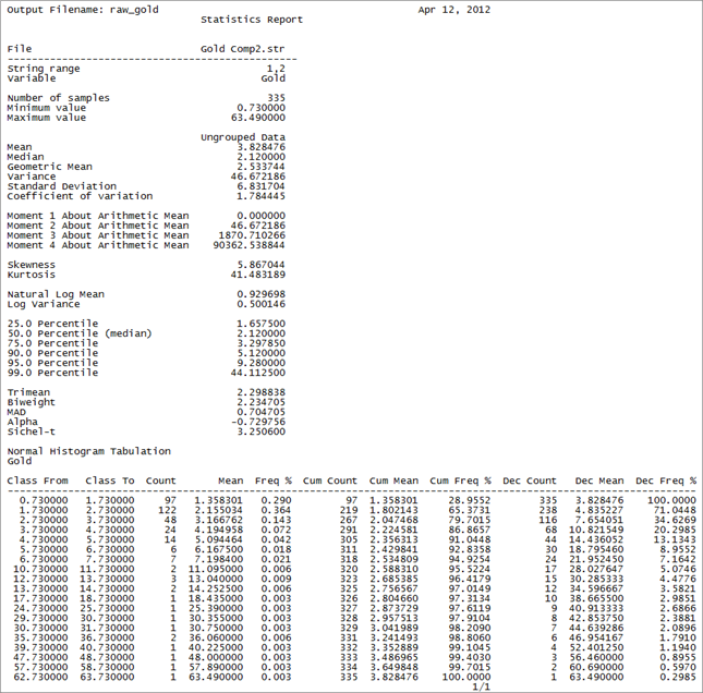
As you can see from the histogram, this distribution is not bimodal. The basic statistics report will be displayed next. Note the values of the mean, standard deviation, and percentiles. |
The output report raw_gold.not is displayed.
Removing Outliers in Surpac
Task: Remove Outliers
Looking back to the histogram of gold_comp2.str, as well as the output report, you can see that the majority of the data is grouped between values of 0 and 10 grams per tonne. Also, you can see that there are several outlier values above 10 grams per tonne.
- Run the macro 08b_cut_outliers.tcl.
- After reading the text below on the first form, click Apply.
- When you have completed viewing the form, click Apply.
- When you have finished viewing the form, click Apply.
- When you have finished viewing the form, click Apply.
- After reading the text below on the next form, click Apply.
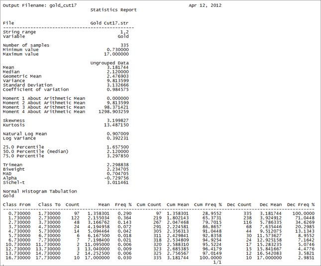
- Open gold_cut17.not and verify that the maximum value is 17.
|
Variograms and subsequent block model estimations are sensitive to outliers (relatively large values). One method of dealing with these data is to reduce, or 'cut' them to some lesser value. The value used to cut outliers can be determined by one of several methods, including: 1. The upper limit of a given confidence interval 2. A given percentile 3. An arbitrarily chosen value
In this example, you will use the value which defines the upper limit of a 95% confidence interval A confidence interval is an estimated range of values which is likely to include a given percentage of the data values. Since a confidence interval is based on the data alone, it is useful where there is little or no knowledge of the deposit. The calculation for the upper limit of a 95% confidence interval (CI) is: 95% CI = mean + (1.96 * standard deviation)
For this data set, mean = 3.828 and standard deviation = 6.831 95% CI = 3.828 + (1.96 * 6.831) 95% CI = 17.217 For simplicity, you will use the nearest integer value of 17 to cut the outlier data. As stated above, other methods can be used to select the outlier cutoff, such as a percentile, or an arbitrarily chosen value. A percentile is that data value at which a given percentage of all other data values fall below. Any given percentile value could be selected as the outlier cutoff, such as the 90th, 95th, or 99th percentile. Recall the following percentile values were given in the basic statistics report: 90th Percentile: 5.120 95th Percentile: 9.280 99th Percentile: 44.112 An arbitrarily chosen value based on knowledge of the deposit and sampling methods may also be used. For example, if part of an ore zone has been mined, information from grade control samples and reconciliation studies may provide a good idea of what the maximum mined block value will be. If the deposit has not yet been mined, information from similar deposits may be useful in dete Whatever method is chosen, values in a description field in a string file can be cut with the use of STR MATHS. |
You run STR MATHS by choosing File tools > String maths.
The String Maths form prompts you to enter the name of the input and output files, as well as an expression. Before viewing this form, the macro has opened gold_comp2.str, and saved it as gold_cut17.str.
The D1 field receives the result of the expression: iif(d1>17,17,d1)
You can reword this expression as:
If the initial value of d1 is greater than 17, then set the value of d1 equal to 17, else leave the value of d1 as it was initially.
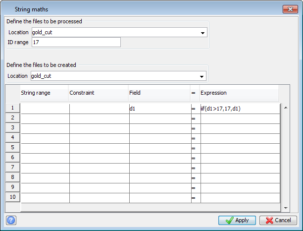
Using string maths to cut outliers
In order to validate the output from STR MATHS, you will analyse the data in the Basic Statistics window. Again, you run this by selecting Geostatistics > Basic statistics.
Next, the macro will choose File > Load data from string files, and the following form below is displayed. Notice that gold_cut17.str is the file being analysed.
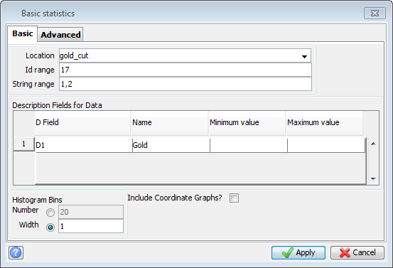
Next, a histogram and a line representing the cumulative frequency is displayed. Notice that the maximum data value is now 17. After this, the macro selected Statistics > Report. This form prompts you to enter the name of an output report, the report format, and a range of percentiles which will be written to the report.
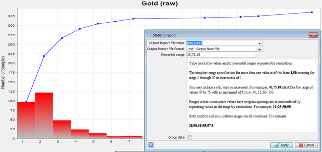
Percentile range definition
|
The D1 field in the file gold_cut17.str contains the D1 values from gold_comp2.str. As displayed by this histogram, you can see that the maximum value is 17.000. The D1 field in gold_cut17.str will now be used for all subsequent variography analysis, as well as block model estimation. |
The output report gold_cut17.not contains several output statistics, including the specified percentiles. This file is created in the directory, but is not displayed by the macro.