Triangulation algorithm function

Function Name:

STITCH ALGORITHM TOGGLE

This section provides an explanation of the Triangulation Algorithm function and how it can be successfully applied in different circumstances.

Choose Triangulation Algorithm from the Triangulate menu to change the triangulate stitch algorithm while Surpac is running.

The stitch algorithm is the algorithm used by the Triangulate functions to create triangles to stitch segments together. You will find that different stitch algorithms will give you better results in different geometric situations. You have four options, which are represented by the integers 0-3 on the Triangulation Algorithm form.

The options are:

0: old algorithm
1: new algorithm
2: old algorithm with transforms
3: new algorithm with transforms

The default value of the option in the defaults.mst file is 3.

Please Note: The old algorithm is the algorithm which existed in Surpac prior to Version 3.0.

Exercise to demonstrate the effects observed with a particular string file of each of the different toggle stitch algorithms.

Recall File `BIFURC2.STR' into GRAPHICS.
Change the view of the data to easily see strings 1 and 2. ie. View by Bearing (alias = VB) bearing = 0 dip = -15

Choose Triangulation algorithm from the Triangulate menu and select new algorithm with transforms. This is the default setting that is suitable for most data sets.

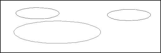
This option uses a recently developed algorithm and has a step which transforms the segments so they are parallel and have aligned centroids before performing the stitching and then removing the transform. This is particularly successful when the data is coplanar but segments are at a high angle to one another.

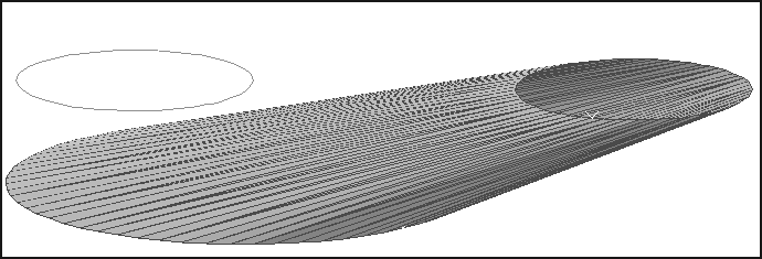
Choose Between Segments from the Triangulate menu and create Object 1 Trisolation 1.
Select string 1 then the right most segment of string 2 as shown:

Note the resultant surface triangulation.

Recall File `BIFURC2.STR' without saving the result from the previous exercise and choose a similar view.
Choose Triangulation algorithm from the Triangulate menu and select old algorithm with transforms.
Select the same segments and observe the result.

Please note that the old algorithm with transforms also achieved a successful result but in a significantly longer time frame. This demonstrates the principal difference between the New and Old algorithms, ie. the new one is faster.

Recall File `BIFURC2.STR' without saving the result from the previous exercise and choose a similar view.
Choose Triangulation algorithm from the Triangulate menu and new algorithm.
Select the same segments and observe the result.

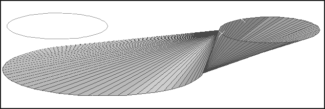
Due to the nature of triangulation algorithms it is sometimes possible for the object to have the minimum surface area but display an unacceptable geometry.

In this case the segments are too far apart geometrically for either the old algorithms or new algorithms (options 0 and 1 respectively) to work and the options with transforms should be chosen in preference.

Finally, choose Triangulation algorithm from the Triangulate menu and reset to new algorithm with transforms.

The principle example where the algorithms without transforms are preferable (ie. options 0 and 1) is when the centroids of the triangulated segments do not approximately align. This happens most often with elongate or lensoid segments or with extremely irregular segments.

Summary

You should now have gained some practice in using the Triangulation algorithm. Note also that the algorithm that best suits your particular data can be set in the Defaults.ssi file as the default algorithm.