The Whittle Interface

Introduction to Three-dimensional Pit Optimisation
Intrinsic Value
Time - The Fourth Dimension
Cost Assumptions
How to Calculate Costs

Block Model Interface

Overview of the Block Model to Whittle Interface
Model Preparation
Required Attributes
Indicator Kriged Models

Block Model to Whittle
Indicator Kriged Models to Whittle
Whittle to Block Model

GEOVIA Whittle is an open pit optimisation and strategic mine planning package. It is not included in Surpac and must be purchased separately. This part of the Surpac package provides you with an interface to Whittle; it allows you to prepare the input files for Whittle from your Surpac geological resource files or block models. It allows you to convert a Whittle result file into a block model. It also allows you to extract Surpac string files from the output of Whittle. You will then use these string files to guide you in your final pit design.

This Whittle interface documentation should be used in conjunction with the appropriate Whittle documentation. The interface documentation will not tell you how to use Whittle but it should give you sufficient information to understand how to prepare your input model correctly for import into Whittle.

Introducing Three-dimensional Pit Optimisation

A number of methods have been described which aim to find the optimal outline for an open pit. Not all methods can guarantee to find the absolute optimum. One method which is guaranteed to find the optimal pit was described by Lerchs and Grossman in 1965, it is on this method that GEOVIA Whittle is based.

The optimal pit outline is the three-dimensional pit outline which, if mined out, would give the maximum currency return whilst still obeying the required pit slope constraints. Consider that every cubic metre of rock in a geological resource model has an Intrinsic Value. If the rock is of a sufficiently high grade, then the value is the price obtainable for the metal which can be extracted from it, less the costs of mining and processing it. If the rock is waste, then the value is negative and numerically equal to the cost of mining it.

The optimal pit outline is thus the outline which maximises the total intrinsic value of the rock included in the outline whilst obeying the pit slopes.

In other words, the optimal pit outline will mine everything that is worth mining. We mine every bit of ore which at any time in the mining process can be mined at a profit. Nothing can be added to or taken away from the optimal outline which will increase the value without breaking the slope constraints.

The Lerchs-Grossman method is a mathematical search technique which works from just two sources of information. The first is a `value' model. This gives the intrinsic value of each of a set of regular rectangular blocks which completely fill the space under consideration for mining. The second is a list of relationships between these blocks. These relationships are known as `arcs'. Each arc goes from one block (A) to a second block (B) and indicates that, if A is mined, then B must be mined first to uncover A. The reverse does not hold since B can be mined without disturbing A. This list of arcs encapsulates the required pit slopes.

Given these two sources of information, a computer program based on the Lerchs-Grossman algorithm will flag each block in the model as being inside or outside the optimal pit outline.

Any feasible pit outline has a Currency Value. By feasible, we mean that it will obey safe slope requirements. The optimal pit outline will be the pit with the highest Currency Value.

Revenue can be calculated from ore tonnages, grades, recoveries and product price. Price is often the biggest unknown but, in order to design a pit, you must assume some price.

In general, if the product price is increased, the optimal pit gets bigger. Similarly, if the costs are escalated, the optimal pit gets smaller. If you use steeper slopes, the optimal pit will generally get deeper. Once all of these factors are fixed, there is only one optimal pit outline.

Costs may be a complex issue but with care, you can calculate the costs of mining and processing to a reasonable level of accuracy.

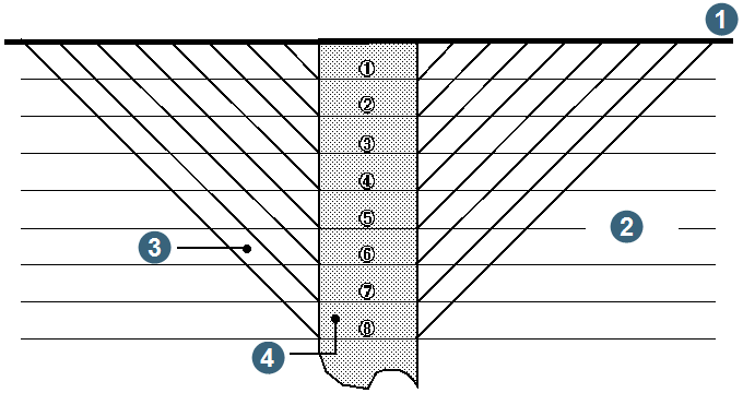
Consider a simple two-dimensional example:

1. surface 2. bench level 3. 100 tonnes waste 4. 500 tonnes ore

Tonnages for possible pit outlines

Pit	1	2	3	4	5	6	7	8
Ore	500	1,500	1,500	2,000	2,500	3,000	3,500	4,000
Waste	100	400	900	1,600	2,500	3,600	4,900	6,400
Total	600	1,400	2,400	3,600	5,000	6,600	8,400	10,400

Pit Values for ore @$2.00/T and waste @$1.00/T

Pit	1	2	3	4	5	6	7	8
Value	900	1,600	2,100	2,400	2,500	2,400	2,100	1,600

Graph showing value (Y axis) and tonnes (X axis)

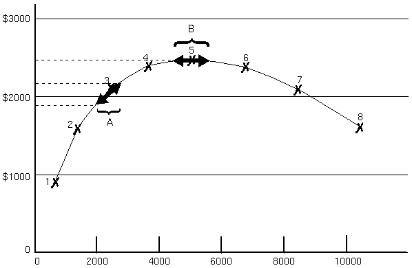
The graph shows that small deviations from a design which is not optimal (A) can have significant effects on pit value. Generations of mining engineers have experimented with small changes to improve their designs. Providing you start from an optimal outline (B), small deviations in the size of the pit will have negligible effect on the value of the pit. The lesson here is that providing your practical design is based on the optimal outline, fine-tuning will be a waste of time. You will gain far more if you examine the sensitivity of the optimal pit to changes in costs or product price.

Open pit optimisation is an iterative process. During sensitivity work, you will explore the economic and slope sensitivity of the resource model. You will get a feel for the general scale of mining and hence the operating costs. You will then decide approximately where the haul roads are going to be and then adjust the slopes in those regions to the average slopes required. There is more to pit optimisation than creating a geological resource model, generating a value model and optimising it, and then doing the final design.

Intrinsic Value

The input model for Whittle is a regular block model which holds data on tonnage and metal content for each parcel of material in a block. Whittle calculates the intrinsic value of each parcel and overall block internally.

There are two basic rules to observe when calculating the value of a block for observation purposes.

First Rule

Calculate the block value on the assumption that it has been uncovered and that it will be mined. When we mine a block, is the grade of any mineralised material in the block high enough to make it worth processing? Make no allowance for average stripping rations because this is precisely what the programs sort out. Take no notice of 'break-even' cut-offs. These are useful for manual design but inappropriate for optimisation purposes. For more information on cut-offs, refer to the section on model preparation.

Second Rule

Include any on-going costs which would stop if mining stopped. This is because when the program is deciding whether to mine a block, it is effectively deciding whether to extend the life of the mine. It must therefore be able to pay for all the costs involved in extending the life of the mine.

Incremental costs such as fuel costs, wages etc. must obviously be included in the cost of mining or processing, whichever is involved.

Overhead costs which will stop if mining stops must also be included. How these should be divided between mining and processing costs is not always easy to determine.

Overhead costs which will not stop if mining stops (such as the repayment of a bank loan) should not be included. They are in effect already spent. If the pit you design will not cover these costs, then the project should not proceed as no amount of design or redesign will make it profitable.

There are a number of ways of writing an expression for the value of a block. The one that Whittle uses is as follows:

where the part of the expression in parentheses is repeated for each separately mineable mineralised parcel in the block for which it is positive, and where:

• ROCK

The total tonnage of the block - not just waste.

• ORE

The tonnage of a particular parcel of mineralised material.

• METAL

The number of units of product in the parcel - this is not the grade.

• RECOVERY

The proportion of product recovered when the material is processed.

• PRICE

The amount of currency obtainable for a unit of the product.

• COSTM

The cost of mining and removing a tonne of waste.

• COSTP

The difference between the cost of mining and processing ore, and the cost of mining waste. (The difference between the cost of mining ore and the cost of mining waste is included in COSTP.)

Air blocks must also be given a value so that the optimisation program can differentiate them from waste. Air blocks have a value of zero. A block can comprise parcels of ore which have a positive value and are worth treating but the block can still have an overall negative value. However this negative value will be less negative than if the block were mined wholly as waste.

The size and shape of an ultimate pit outline is affected more by the economic conditions when mining ends than the economic conditions when mining starts. If the mine life is to be only a year or two, then you can probably predict the economic conditions reasonably well. Otherwise you have a problem.

You can see from formula (1) above that there are three relevant economic variables. These are PRICE, COSTP and COSTM. This of course assumes that the geological resource model has been developed by a competent person with appropriate and adequate information.

If we are to do a thorough analysis and explore the possible effects of varying economic variables, you could look at a range of values, say 10, for each of these variables. This require 1000 individual optimisations.

This is a daunting task. The computation involved in the 1000 optimisations should not be taken lightly, however it is possible. The most significant problem you would be faced with is how to compare and analyse 1000 different pit outlines.

Time - The Fourth Dimension

Whittle gives you the ability to examine your geological resource in the fourth dimension, that is you can consider the effects of sequencing and scheduling.

The effect of time on the value of money

A unit of currency we have today is more valuable to you than the unit of currency that someone is going to give you in a year's time. There are several reasons for this some of which are as follows:

• Inflation will reduce the value of next year's unit of currency - it will buy less.
• If you get the unit of currency now, there is no risk of something going wrong and you not getting it.
• If you have not got the unit of currency now, you may need to borrow it and pay interest on it until you can repay it.

The accepted method to allow for this is to discount next year's unit of currency by a certain amount and cumulatively thereafter for years into the future. This means that you discount future revenues and costs by a particular discount rate and reduce them all to a `net present value' or NPV.

There are two discount rates. The first is the 'notional' discount rate which is applied to actual revenues and costs which are likely to occur. In other words the revenues and costs will follow the inflation rate. Thus the notional discount rate will include an allowance for inflation, and it would be correct to use this provided you inflate all your costs and revenues for future years. It is difficult to guess the future inflation rate.

For this reason it is easier, and most importantly probably more accurate, to work out revenues in today's unit of currency and then to use the second discount rate which is referred to as the

'real' discount rate. The real discount rate takes no account of inflation.

The effect of mining sequence on the optimal pit outline

This is best explained with the aid of Figure 1.

There are two extreme approaches that you can take when scheduling a pit. The first we will refer to as 'flat mining'. This is where you mine all the top bench to the final pit outline, then move your equipment down to the next bench and repeat the exercise and so on. Waste at the top of the outer shell is mined early and the cost is discounted less than the revenue from the corresponding ore which is mined at the end of the pit life. The optimal pit for flat mining is thus generally smaller than would be indicated by simple optimisation using today's costs and revenues.

The second approach is 'incremental' mining where each shell is mined in turn and thus the related ore and waste is mined in approximately the same time period.

Figure 1 has introduced the concept of incremental or 'nested' pits. A series of value models may be prepared for, say, a range of product prices. The outlines obtained from putting these through a three dimensional optimiser will form a set of nested pits.

The only problem here is that you want to maintain your usual high professional standards and will therefore need to look at a range of processing and mining costs, and all the interactions between the different costs. You have just presented yourself with the 1000 pit problem.

A modified block value formula can reduce the size of the problem.

If, for a given set of economic value, you calculate a set of block values, in say dollars, you will get a particular value for each block. If you Then run these values through an optimiser, you will get a particular pit outline. If you then calculate the block value in cents, the numeric value allocated to each block will be one hundred times bigger. If these values through an optimiser, the pit outline we get will be identical to the one we got when we used dollars. Now, if you calculate the block value in Roubles....

In other words, we can use any money as our unit of currency and you will always get the same optimal pit outline. What matters is the ratios between the block values, not the values themselves.

Given that PRICE, COSTP and COSTM are each amounts of money (e.g. dollars/oz, dollars/tonne etc.), then any of them could be used as a unit of currency. However, there are particular advantages to using COSTM as the unit of currency. If we divide all the terms of our Value formula by COSTM, it becomes:

There are now only two economic variables. These are (PRICE/COSTM) and (COSTP/COSTM). Now you only need to do 100 optimisations to maintain your professional integrity!

If you examine the economic variable (COSTP/COSTM) more closely, you will see that it is the ratio between the cost of processing ore and the cost of mining waste. Four-D calls this cost ratio the CRATIO and experience will show that this ratio is surprisingly stable with time.

The block value formula becomes:

If fuel costs increase, the haulage costs for ore and waste will both be affected. If labour costs change, they are likely to change for employees working in both the processing plant and the mine.

Although the CRATIO is an economic variable, it is not really an economic unknown if you break your costs down correctly. For many purposes the CRATIO can therefore be regarded as fixed. This is good news because now instead of 100 optimisations, you need only do 10.

Remember that although the CRATIO is stable with time, it can certainly vary with position in your pit.

It is hard to relate to the economic variable (PRICE/COSTM). However, if you invert it to give (COSTM/PRICE) this is the amount of product you will need to sell to pay for the mining of a tonne of waste. It will henceforth be referred to as the metal cost of mining (MCOSTM). It has the units of a grade, but this is not the grade which has anything to do with ore grades. In a large open pit gold mine for example, it may be 0.1 grams per tonne or 0.03 ounces per ton.

The final form of the block value formula becomes:

CRATIO is reasonably stable

MCOSTM is dependent on prices and costs

Although we have reduced the number of unknown variables from three to one, there is no loss in generality between formulae (1) and (4)

By using formula (4) for the block values and stepping MCOSTM over a suitable range of values you can generate a series of value models which can then be optimised with a three dimensional optimiser to produce a series of pit shells similar to the ones in the simple example, but for a real geological resource model.

Four-D automates this stepping and optimising process and the way that you can use the resultant pit shells is what sets Four-D apart from Three-D.

Since each shell honours the required pit slopes, you can use the shells to indicate technically feasible mining sequences. Four-D will allow you to analyse three separate sequencing scenarios.

Worst Case Scenario

In this, Four-D completes the mining of each bench before starting the next bench. This is well known to be the worst way of making money out of a pit, although in some small pits, it may be the only practical course available.

Since it is the worst, it sets a floor on the NPV.

The precise sequence used by Four-D is to mine the top bench of the smallest of the pit shells, followed by the strip between the smallest and the next smallest etc. until the ultimate pit has been reached. After this the process is repeated for the second bench.

Best Case Scenario

In this, Four-D mines the pit as a series of narrow push backs, often thirty or forty. This is rarely physically feasible, because the push-backs are usually far too narrow. But, if it were practical, and if mining this way did not increase the costs, it would provide you with the best possible early cash flow.

Since it is the best, it sets the ceiling on the NPV of the pit.

When the worst and best NPVs are very similar, as they may well be in a small mill-limited operation with a fairly even grade, then you can conclude that the mining sequence has very little effect on the NPV and can therefore be ignored for design purposes.

Specified Push-Back Scenario

The actual mining sequence will lie somewhere between the worst and best case sequencing scenarios. Four-D will allow you to select particular pit shells as push-backs. Thus practical push-backs can be considered and the effect they have on the cash flow and NPV assessed.

Cost Assumptions

There are three basic rules to follow when you calculate the value of a block for optimisation purposes.

The First Rule

The value must be calculated on the assumption that the block has already been uncovered. In other words no allowance should be made for the cost of the stripping required to access the block, because this is precisely what the optimiser calculates. In particular, any cut-off used to define ore should reflect the cost of processing and any extra cost of mining the block as ore rather than waste, but not the cost of stripping. If an allowance for stripping is included in the costs, the stripping will be paid for twice.

The Second Rule

The value should be calculated on the assumption that the block will be mined. So, if the block contains some ore that could be profitably be processed as well as some waste, the value of the ore should be added in, even if the net value of the block is still negative. The optimiser will chose to mine such a block, but if it has to mine it to get to a more valuable block, the ore will help pay for the stripping, as it would in practice.

The Third Rule

Any cost that would stop if mining stopped must be included in either the cost of mining or the cost of processing. Conversely, any cost that would not stop if mining stopped must be excluded. This is discussed in more detail later on.

How to Calculate Costs

It was stated above that any cost that would stop if mining stopped must be included in the cost of mining or the cost of processing.

The reasoning behind this is that, when the optimiser adds a block to the pit outline, it may effectively extend the life of the mine. If the extra overheads involved in this are not included when calculating the block value, then the addition of a positive block may actually reduce the value of the pit.

All day-to-day costs such as wage and fuel costs must, of course, be included, and it is usually clear whether they should be included in the mining or the processing cost. However, there are some costs where the correct treatment is not so obvious. Some examples of the handling of various costs may be helpful:

Processing Mill

Consider a processing mill and mine infrastructure that costs $50 million to build and commission.

If the mine were to shut down, for whatever reason on day 2, the mill and infrastructure would have a certain salvage vale, say $30 million. In this case, $20 million has gone forever. It is an up-front or sunk cost that must be subtracted from any optimised value of the pit itself.

You can deal with the $30 million in two ways.

If we assume that there will be an on-going program of maintenance and capital replacement that will keep the salvage value of the mill close to $30, then the $30 million is theoretically recoverable when the mine closes, and so is not a cost. However, the maintenance and periodic capital replacement expenses are costs for these purposes, because they would stop if mining stopped. They should be averaged and reduced to a figure per ton processed. This figure should be added to the direct costs of processing, such as wage and fuel costs.

Alternatively, you could assume that only essential maintenance will be done and that the salvage value of the mill will progressively decline. In this case, the expected rate of decline should be added on a per ton basis to the essential maintenance, wage and fuel costs. Note that the rate of decline is not necessarily the rate of depreciation used by accountants. In most cases, the depreciation rate is set by a taxation regime, and may reduce the book value to zero when the salvage value is clearly not zero.

To reduce costs to a per ton basis, assumptions have to be made about the production rate. If the size of the pit produced by the optimisation makes these assumptions inappropriate, then the costs must be recalculated and the optimisation done again. You should set up all your cost calculations on a spreadsheet, this makes the recalculation much easier.

Trucks

If the expected life of the mine is shorter than the operating life of a truck, then the truck purchase must be treated in the same way as the cost of the mill, except that it will probably be included in the mining rather than the processing cost.

If the life of the mine is much longer than the life of a truck, then the trucks will have to be purchased progressively to maintain the fleet, and such purchases will stop if mining is stopped. Consequently the cost of purchasing trucks should be averaged out over the life of the mine and reduced to a cost per tonne.

Unless the life of mine is expected to be very long, some compromise between the above two approaches is usually required.

Contract mining companies must take these factors into account when quoting for a job, and it sometimes useful to think as they do when working out the cost of a company owned fleet, except that the contractor's allowance for profit is not included.

Administration Costs

On-site administration will usually stop if mining stops. They must therefore be included somewhere in the costs. The question is should they be included in the mining or processing cost?

The answer depends on whether production is limited by mining or by processing. Usually, it is limited by processing, and in this case only the mining of an ore block extends the life of the mine. The ore block values should therefore include an allowance for on-site administration costs. The cost is, in effect, added to the processing cost per ton. Conversely, if production is limited by mining, as in a heap leach operation, every block that is mined extends the life of the mine, so that on-site administration costs should be added to the mining costs.

Head office administration costs may or may not stop if mining stops, and thus may or may not be included.

Bank Loans for Up-Front Costs

Repayment (principal and interest) of a bank loan taken out to cover up-front costs will have to continue whether mining continues or not. It should therefore not be included in the costs used for calculating block values.

Of course these payments have to come from the cash-flows of the mine. If the mine is not going to produce enough cash flow to cover them, the project should not proceed. These repayments should not be introduced as costs in an attempt to `improve' the optimisation. The result will in fact be quite the opposite - a smaller pit with a smaller total cash-flow.

Although the bank loan repayments themselves are not included, some items that the loan was used to pay for may be included as you will see below.

Bank Loans for Recoverable Costs

If money is borrowed from the bank for day-to-day working capital or for items such as the $30 million discussed in the mill example above, then the salvage value can be realised and repaid to the bank if mining stops. Consequently the interest paid on such a loan is a cost that stops if mining stops. It should therefore be treated as an overhead like the on-site administrative costs discussed above.

Grade Control Costs

It is usually necessary to do grade control work on waste as well as ore. In this case grade control costs apply to waste costs too. If only some of the waste is grade controlled, then you can either load the cost of those particular waste blocks, or make an estimate of the tonnes of such waste per tonne of ore, and load the cost of mining ore.

Support - Cable Bolts

The cost per tonne is related to the pit size, which has to be calculated by the optimiser. Then a cost per unit of area of wall can be transformed into a cost per tonne of waste. This is an iterative estimate, but fortunately costs per tonne are usually low.