


GSLIB Sequential Gaussian simulation
To run this function: Choose Block model > Estimation > GSLIB > Sequential Gaussian simulation, or...
Files Tab
Input
Location, ID number, String range, D-field, Weight
You must complete each of these inputs to describe the string file or files from which the sample data is to be obtained. Enter the Location and Id range of the required string file. Enter the String range and the description field(s) to define the data from the string file which are to be used for estimation. The specified data will be converted from a string file to the geoEAS format input file that GSLIB requires.
The declustering weight field can be left blank if there aren't any declustering weights.
Minimum
All samples strictly less than this value are ignored. An example value is -1E+21.
Maximum
All samples strictly greater than this value are ignored. An example value is 1E+21.
Output
Estimate
Specify a block model attribute prefix. This will be combined with each realization number to create the attribute names that store the results of each realization. For example, if you specify a prefix of gold and four realizations, the attributes used will be gold1, gold2, gold3 and gold4.
Number of realizations
Specify the number of realizations. Each realization creates a unique set of estimates. An example value is 1.
Seed
A random number seed (a large, odd integer).
Constrain interpolation
If you want to estimate a subset of the block model blocks by use of a block model constraint, check this box.
Debug file
The name of the GSLIB debug file to create.
Debug level
The higher the debugging level, the more output. The normal levels (none, low) summarize the results. Medium and high provide all the kriging matrices and data used for the estimation of every point/block. It is recommended that a high debugging level not be used with a large block model.
Clean up
When the form is Applied, a number of (temporary) files are created, either for input to GSLIB or as output from GSLIB. If you check this box, the temporary files will be cleaned up (deleted).
Transformation Tab
Transformed
Check this box if the data is already standard normal. Leave the box unchecked to transform the data.
Min data value
The minimum data value allowed, for example 0.
Lower tail
Select the method of interpolation to the lower limit.
w
Specify the power model parameter, for example 0.
Max data value
The maximum data value allowed, for example 0.
Upper tail
Select the method of interpolation to the upper limit.
w
Specify the power or hyperbolic model parameter, for example 1.
Smooth the distribution
Check this box if you want to consider a smoothed histogram of the data for transformation.
Scaling type
Select whether to perform arithmetic or logarithmic (base 10) scaling
Number of Z values
The number of evenly spaced z values for the smoothed histogram, for example 100.
Minimum Z
The lower limit of the evenly spaced z values, for example 0.0.
Maximum Z
The upper limit of the evenly spaced z values, for example 1.0.
Max Perturbations
After Number of Z values x Max Perturbations perturbations, smoothing is stopped. An example value is 750.
Report after
After Number of Z values x Report after perturbations, the current objective function(s) are reported. An example value is 50.
Min objective
When the normalised objective function reaches this value, smoothing is considered complete. An example value is 0.0001.
Smoothing window size
The size of the smoothing half-window. An example value is 5.
Closeness to target mean
Check this box if you wish to consider closeness to a target mean.
Weight
The weight that scales the automatically calculated weight for closeness to a target mean.
Closeness to target variance
Check this box if you wish to consider closeness to target variance.
Weight
The weight that scales the automatically calculated weight for closeness to a target variance.
Closeness to target smoothness
Check this box if you wish to consider closeness to target smoothness.
Weight
The weight that scales the automatically calculated weight for closeness to target smoothness.
Closeness to specified quantiles
Check this box if you wish to consider closeness to specified quantiles.
Weight
The weight that scales the automatically calculated weight for closeness to specified quantiles.
Specify mean
Check this box and enter a target mean if it is different from the mean of the data.
Specify variance
Check this box and enter a target variance if it is different from the variance of the data.
Quantiles from data
The number of quantiles defined from the data. An example value is 5.
User defined quantiles
cdf
z
Specify quantiles consistent with the data to control peaks and troughs in he smoothed distribution.
Simulation Options Tab
Kriging Type
Specify which type of kriging to use.
- Simple kriging
- Ordinary kriging
- Simple kriging with a locally varying mean
Mean attribute
A gridded data file (.grd) will be created. The value of the specified attribute will be written for each user block to be estimated. These means will be used in the Simple Kriging of each block.
Kriging with an external drift
Drift attribute
A gridded data file (.grd) will be created. The value of the specified attribute will be written for each user block to be estimated. These external drift values will be used for non-stationary kriging.
Drift D-field
The field in the input string file containing the external drift values to use for non-stationary kriging.
Collocated kriging with one secondary variable
Secondary attribute
A gridded data file (.grd) will be created. The value of the specified attribute will be written for each user block to be estimated. These secondary sample values will be used for collocated kriging.
Correlation coefficient
The correlation coefficient between the primary and secondary variable.
Variance reduction factor
This factor reduces the kriging variance after collocated cokriging. The default is 1.0 (unchanged).
Maximum samples per octant
The maximum number of samples per octant (octant search is not used if this value is left at 0). The octant search ensures that data are taken on all sides of the point being estimated. This is particularly important with drillhole data. An octant search ensures that data is sourced from more than one drillhole. An example value is 12.
Number of simulated nodes to use
The maximum number of previously simulated nodes to use for the simulation of another node.
Multiple grid search
Check this box to perform a multiple grid simulation. Leave the box unchecked to perform a standard spiral search of previously simulated nodes.
Number of multiple grid refinements
The number of multiple grid refinements to consider. An example value is 3.
Assign data to nodes
If this box is unchecked, the data and previously simulated grid nodes are searched separately: the data are searched with a super block search and the previously simulated nodes are searched with a spiral search. If the box is checked, the data are relocated to grid nodes and a spiral search is used (the parameters Minimum samples to krige a block and Maximum samples to krige a block are not considered).
Minimum samples to krige a block
The minimum number of data points to use for kriging a block. If fewer than this number of samples are found, the block will be left unestimated. An example value is 4.
Maximum samples to krige a block
The maximum number of data points to use for kriging a block. For example, specifying 8 uses the closest eight sample points to the centroid of the block being sampled.
Search radius
The search radius in the maximum horizontal direction (hMax), the minimum horizontal direction (hMin) and the vertical direction (Vert). See Ellipsoid Definition for more detail on specifying these radii. An example value for each direction is 20.
Search angles
The angle parameters that describe the orientation of the search ellipsoid. See Ellipsoid Definition for more detail on specifying these angles. An example value is 0.
Size of covariance lookup table
Enter the X, Y and Z dimensions of the covariance lookup table. Example values are X 9, Y 8, Z 11.
Variograms Tab
An acceptable variogram model for GSLIB consists of a nugget effect and any positive linear combination of standard variogram models: spherical, exponential, gaussian or hole effect.
Nugget
Specify the nugget constant for the variogram. An example value is 1.
Type
Select the type of structure represented by this line of the table. The structure types supported by GSLIB for Indicator Kriging are:
- Spherical
- Exponential
- Gaussian
- Hole effect
Cc
Specify the c parameter for this structure. An example value is 1.
hMax
An example value is 1.
hMin
An example value is 1.
Vert
The maximum horizontal range, minimum horizontal range and vertical range. See Ellipsoid Definition for more detail on specifying these values. An example value is 1.
Angle1
An example value is 0.
Angle2
An example value is 0.
Angle3
Specify the angles defining the geometric anisotropy. See Ellipsoid Definition for more detail on specifying these angles. An example value is 0.
Post Processing Tab
Post processing is possible for simulated data.
Output type
Select whether to compute:
E-type estimate and conditional variance, i.e., the mean value of the conditional distribution and conditional variance of the conditional distribution.
Estimate
Specify a block model attribute to store the estimate.
Conditional variance
Specify a block model attribute to store the variance.
Probability and means above and below ... a fixed threshold,
Threshold
The Threshold of interest.
probability > Threshold
Specify a block model attribute to store the probability of exceeding the threshold.
mean > Threshold
Specify a block model attribute to store the mean value above the threshold.
mean < Threshold
Specify a block model attribute to store the mean value below the threshold.
Z percentile corresponding to ... a fixed conditional cumulative distribution function (cdf) value,
cdf
The cdf value of interest.
z value
Specify a block model attribute to store the z value.
Symmetric probability interval with width...
Total width
The total width of the interval.
Lower, Upper
Specify block model attributes to store the symmetrical probability interval.
Results
Press Cancel to cancel the function or Apply to invoke GSLIB.
The flow of data is:
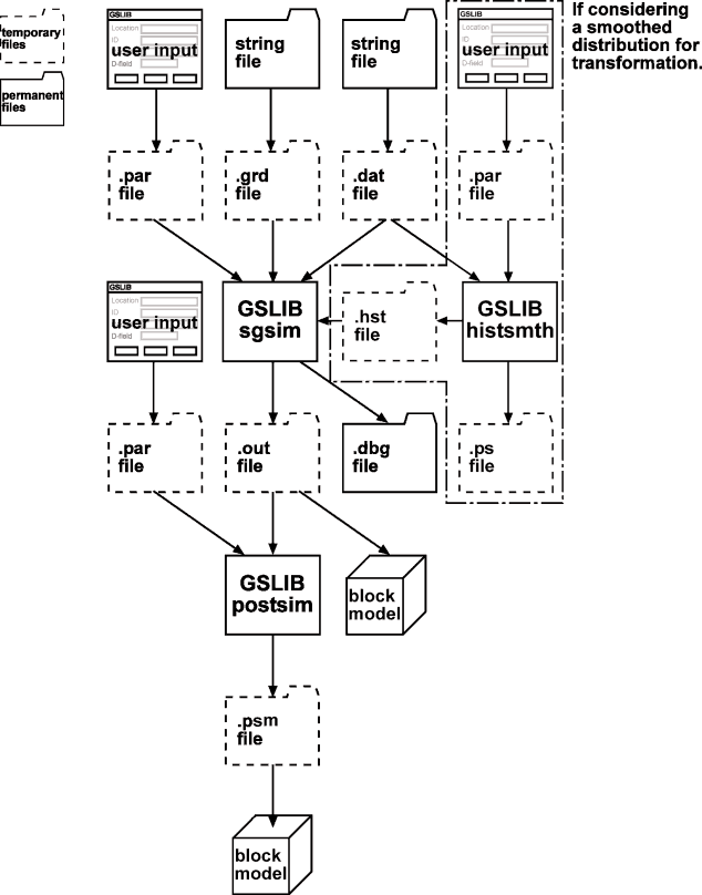
Sequential Gaussian simulation with GSLIB is a two or three step process:
- If you need GSLIB (sgsim) to transform your data and you want to use a smoothed reference distribution for this process, GSLIB (histsmth) requires the sample (.dat) file and a parameter (.par) file.
The sample (.dat) file is created from the specified string file and the form input is used to create the parameter (.par) file.
The file names are created from the location of the sample file and the relevant file name extension.
GSLIB (smthhist) creates two files, a (.hst) file of the smoothed histogram and a (.ps) plot file of the histogram. The smoothed variogram is automatically loaded into GSLIB (sgsim) when the transform is performed. The GSLIB screen output is written to the message window prefixed with:
GSLIB>
If the data is already transformed or you don't want to consider a smoothed histogram, this step is skipped.
- GSLIB (sgsim) requires a sample (.dat) file, a parameter (.par) file and (optionally) a .grd file of gridded data (if you are performing Simple kriging with a locally varying mean, Kriging with an external drift or Collocated kriging with one secondary variable).
The sample (.dat) file is created from the specified string file, the form input is used to create the parameter (.par) file and the gridded data is extracted from the block model.
The file names are created from the location of the sample file and the relevant file name extension.
GSLIB (sgsim) creates two files, a (.out) file of simulated results and a (.dbg) file with information about the simulated results. The simulated results are automatically loaded into the specified block model attribute(s). The GSLIB screen output is written to the message window prefixed with:
GSLIB>
After GSLIB (sgsim) has finished kriging, further post processing can be performed by GSLIB (postsim).
- GSLIB (postsim) requires a GSLIB (sgsim) output (.out) file and a parameter (.par) file.
The GSLIB (sgsim) output (.out) file is created by GSLIB (sgsim) and the form input is used to create the parameter (.par) file.
GSLIB (postsim) creates one file, a (.psm) file of results. The results are automatically loaded into the specified block model attribute(s). The GSLIB screen output is written to the message window prefixed with:
GSLIB>
If you selected Clean up on the Files tab, the temporary files will be deleted after the results have been loaded into the block model.
Messages
Removing GSLIB intermediate files.
You selected Clean up on the Files tab, so the temporary files created for or by GSLIB are being removed.
Error loading file filename0.str
There was an error loading the specified string file.
You must select a model first.
You must open a block model before you can use this function.
File c:\Program Files\Gslib90\sgsim.exe not found
File c:\Program Files\Gslib90\postsim.exe not found
File c:\Program Files\Gslib90\histsmth.exe not found
sgsim.exe, postsim.exe or histsmth.exe could not be found in the specified directory. Make sure the gslib90 user option is pointing to the directory containing sgsim.exe.
Invoking "c:\Program Files\Gslib90\histsmth.exe" sample2.par ...
Invoking "c:\Program Files\Gslib90\sgsim.exe" sample.par ...
Invoking "c:\Program Files\Gslib90\postsim.exe" sample3.par ...
sgsim.exe, postsim.exe or histsmth.exe is being invoked with the specified parameter file.
You have terminated "c:\Program Files\Gslib90\histsmth.exe" sample2.par. Results were not loaded.
You have terminated "c:\Program Files\Gslib90\sgsim.exe" sample.par. Results were not loaded.
You have terminated "c:\Program Files\Gslib90\postsim.exe" sample3.par. Results were not loaded.
You chose to abort the simulation process. This terminated the executable using the progress feedback cancel button before the results were loaded.
"c:\Program Files\Gslib90\histsmth.exe" sample2.par terminated prematurely.
			Results were not loaded.
"c:\Program Files\Gslib90\sgsim.exe" sample.par terminated prematurely. Results were not loaded.
"c:\Program Files\Gslib90\postsim.exe" sample3.par terminated prematurely. Results were not loaded.
sgsim, postsim or histsmth crashed or otherwise ended prematurely (for example, it was terminated outside of Surpac by using Task Manager) before the results were loaded.
Error writing file "sample.dat".
Error writing file "sample.par".
Error writing file "sample2.par".
Error writing file "sample3.par".
An error occurred while writing the specified file. Check that there is enough room to write the file.
Error opening file sample.dat
Error opening file sample.par
Error opening file sample2.par
Error opening file sample3.par
An error occurred while trying to open the specified file for writing. Check that the file is not read-only or in use by another process.
Error opening file sample.out
Error opening file sample.psm
An error occurred while trying to open the specified file for reading. Check that sgsim.exe did not end prematurely and that the file is not in use by another process.
Created sample.dat.
Created sample.par.
Created sample2.par.
Created sample3.par.
The specified file was successfully created.
You have terminated the loading of results. Results were only partially loaded.
You chose to abort the block model loading process.
Number of blocks estimated 4096
The number of blocks actually informed is reported.
Attribute mean does not exist
The specified block model attribute does not exist. Select a different Mean, Drift or Secondary Attribute.