Block models

The Block Model is a form of spatially-referenced database that provides a means for modelling properties of a user-defined volume by amalgamating data and objects into a common space. Information contained in the Block Model is referenced through its intersection with spatial objects (digital terrain models, three dimensional models, plane surfaces, etc.), or interactively using the mouse.

Records in the Block Model are related to discrete volume elements or blocks. These are cuboid partitions of the modelled space and are created dynamically according to the operations performed on the Block Model. Each block assumes values for each of the properties to be modelled. These values apply to the entire volume represented by each block in contrast to a gridded model where such values are related to a point. The properties or attributes may comprise numeric or character string values.

Information contained in the Block Model may be retrieved as text reports or string files, or may be accessed interactively in the Graphics module where colour coded representations of the model may be viewed and individual blocks edited.

All Block Model functions may be performed with constraints. A constraint is a logical combination of one or more spatial objects using logical operators, and which are intersected with the model to allow operations on selected blocks. Objects that may be used in constraints are plane surfaces, digital terrain models, three dimensional (wireframe) models, closed strings and blocks. Constraints may be saved to a file for rapid re-use and may themselves be used as components of other constraints.

Features of the Block Modelling Module

Graphics presentation

3-D visualisation is becoming more widely recognised as an effective method to communicate ideas and concepts to non-technical people. The Block Model can be viewed using variations on two basic methods each of which provide you with all the flexibility you will ever require for visualising a Surpac Block Model. These methods are:

1. Viewing the blocks which meet some simple or complex combination of constraints. This permits you to easily view blocks whose rock type is `X' for example, alternatively it is just as easy to view all blocks for which a numeric attribute is greater then a desired cut-off value.
2. The location of one or more sections can be easily described using the mouse. Sections, actually slabs of some user defined thickness, will be then drawn immediately for viewing.

In both cases different colours can be used to represent ranges of numeric values for an attribute field or different rock types by performing character comparisons.

Rotation

The block model can be used to correctly model a dipping ore body, by enabling it to rotate in three dimensions. All other block model functions can be performed on the rotated model, allowing you to extract sections, report and constrain (for example) on elevations.

Dynamic addition of attributes

At the time when you create the model it is unlikely that you will foresee the various uses to which the model may be put during the life of the model. The ability to dynamically add and remove attributes from the model provides you with the flexibility to use the model for a myriad of purposes which you may not have even considered when the model was initially created.

Calculated Attributes

Calculated attributes are attributes whose values are calculated from the values of other attributes in the model. They are calculated on demand (ie when the value is needed) and as such are always fully up to date, with no interaction by the user necessary. They take up effectively no storage space.

Calculated attributes can be created using Surpac's standard generic expressions, which are the same as any expression possible with BLOCK MATHS.

Filling the model with values

Individual blocks within the model must, at some point, have values assigned to the various attribute fields which exist in the model. A number of methods are available to aid in completing this task. These methods include simple techniques such as Nearest Neighbour interpolation and Direct Assignment through to more complex techniques such as Inverse Distance and Kriging using Variogram estimators.

Constraints

Probably the most powerful feature of the Block Model is its ability to apply both simple and incredibly complex constraints to the model to assist in all aspects of modelling including, filling the model with values, reporting, graphics visualisation, sectioning the model, etc. The constraints may take the form of DTMs, 3DMs, strings and planes of any orientation. These constraints may be applied to the model individually, or they may be combined using a logical expression of the form "((a AND b) OR (c AND d))" etc. These constraints may take some time to create and so it is possible to save the constraints to a Constraints Model for later use. The Constraints Model is in reality just another Block Model with only the blocks which meet the constraints criteria actually being stored. The advantage gained by storing the constraints to a separate model is that later re-application of the Constraints Model is extremely fast.

Constrained block models

Block models with very high resolutions can become very large as more data is added. If only a part of a model is of interest then it can be loaded under constraints to reduce the amount of information loaded. This can significantly reduce the memory overhead of the model and speed up operations on the block model. As an example, we may only be interested in the data between two northings and can load only the parts of the model between these northings.

Constrained models can also be merged back to the original model thus providing a convenient means of dealing with large models.

Sections through the model

Representation of geological structures and grade distribution on vertical, horizontal or oblique sections have long been used as an aid to interpretation of those structures. It is possible to produce such sections from the Block Model on section planes of any orientation. The resultant sections contain string outlines to show where the various physical blocks from the model have been intersected by the section plane. These sections (string files) can then be used by any of the other modules available for further processing.

Reporting

The powerful 3-D visualisation capabilities available in the Block Model make it possible to visually inspect the model in a variety of graphical presentations. It is essential however to be able to examine the resultant model in purely numerical fashion, especially when you consider that one of the prime reasons for using the Block Model is to determine volume, mass and total as well as average content of metal or contaminant. The Block Model contains a flexible reporting function which permits you to produce such reports with results grouped and ordered by various attributes stored in the Block Model.

Super Blocking

In an attempt to conserve memory as much as possible, the Block Model will minimise the number of blocks required to accurately represent the volume of space being modelled. This is done by aggregating (super blocking) a number of adjacent blocks into a single larger block when all of the adjacent blocks have exactly the same value for all attributes which exist in the model. Super blocking will only occur if neighbouring blocks all share the same attribute values. Super blocking will occur recursively until no more blocks can be aggregated into a single block.

This can work differently, depending on the sub blocking scheme you have chosen to use. Using a standard sub blocking scheme, a block will only be super-blocked if all 8 adjacent blocks have the same value. When using a variable sub blocking scheme, small blocks may be super-blocked if 2, 4 or 8 adjacent blocks have the same value. The number required to super block is entirely dependant on your minimum block size and the size of the blocks being tested for super-blocking.

Applications for the Block Model

The Block Model is ideally suited to volumetric modelling for many different purposes and should be used by many different disciplines as an aid to solving complex modelling problems encountered by the various Earth Resources disciplines including, Surveying, Geological Modelling and Evaluation of Ore Reserves, Mine Planning, Groundwater Modelling, Contaminant Remediation, Waste Disposal, etc.

Some classic examples of the use of the Block Model are described briefly below.

Ore resource evaluation

Probably the Classic application of the Block Model. The Block Model is used here to estimate volume, tonnes, total and average metal content of one or more elements of interest. The model is typically constrained by structural elements generally defined either by DTMs or 3DMs or string outlines on vertical or horizontal planes. Reports produced are useful for economic evaluation of potential mines for either surface or underground mining operations.

Modelling of stockpiles

An unusual application for the Block Model and one which will be readily accepted by the surveying profession. Surveying of stockpiles is a relatively trivial exercise if you are only concerned with the volume of material in the stockpile. Techniques involving aerial photogrammetry/electronic theodolites and Digital Terrain Modelling ensure that the volume calculations have small margin for error and that calculation time is minimal. The determination of the content, that is the average grade, of the material in the stockpile, especially if the stockpile is expected to have a long life (of the order of years), is more difficult.

The problem, when considered carefully, is no different to the ore resource evaluation exercise described above. To explain in more detail, consider the application of the Block Model using the following steps:

1. As material is added to the stockpile, surveys could be conducted to define the new surface, or at least the area of change.
2. From these surveys a DTM may be formed, and the blocks above the previous surface and below the current surface tagged with identifying codes to describe various attributes such as the date of the survey, and most importantly, the grade of the material being placed in the stockpile.
3. Over time a reasonably precise model of both the volume and the grade of the stockpile will eventuate.
4. At some future date as material is removed from the stockpile a precise estimate of volume and grade is easily determined by conducting surveys of the material removed and simply reporting the volume, tonnes and grade of the blocks which have been moved.

Modelling of land fill for waste disposal

This application is in essence quite similar to the example described above for stockpile modelling. It differs however in that generally the land fill is intended as a permanent feature rather than being temporary as is the case with a stockpile. With environmental concerns becoming more prevalent it is essential, mostly due to government regulations, that the managers of land fill sites be able to record the composition of the material being placed in the land fill. By using the techniques described this becomes a simple exercise and furthermore, if the procedures described above are followed, it becomes a trivial exercise to visualise, using 3-D graphics, the contents of the land fill site as well as produce printed reports of the land fill content.

Block Model Concepts

Current model

You may have many Block Model files but you may only work on one model at a time. This model is referred to as the `Current Model' throughout this manual. To make a model become the Current Model you must either enter the model name after choosing the BLOCK MODELLING button from the main menu or by choosing the Select Model buttons from the BLOCK MODELLING menu.

User block size

User block size is the block size at which estimation is performed. The user block size provided at the time of model definition and creation is used to provide a constant size target for the numerical interpolation methods and to allow you to relate the size of the model to the number of blocks that comprise the model. Blocks of these precise dimensions rarely exist as the model will create blocks of varying sizes to ensure that constraints which are applied to the model are represented as precisely as possible within the resolution limits of the model. Thus, blocks whose dimensions are equal to the user block size are generally referred to within this manual as virtual blocks since they (generally) don't really exist.

Conditions under which blocks of user block dimensions will actually exist are when the extents of the model and the model resolution relate to each other such that:

user block size = model extents/model resolution

e.g. If the user block size = 10 x 10 x 10 and the model extents are 1280 x 1280 x 1280 and the model resolution is 128 maximum blocks per side, then the smallest blocks which can be represented in the model are 10 x 10 x 10. This does not guarantee that all blocks will be 10 x 10 x 10 as blocks of larger sizes may suffice in some areas depending on constraints which are applied during the course of processing the model.

Virtual blocks

These are blocks which don't really exist in the model. That is, storage space is not allocated for these blocks but reports can be produced, either printed or in the form of string outlines in string files, which provide details of virtual blocks. This concept is important as blocks of the user block size are generally virtual blocks and so there is an internal and transparent aggregation of physical blocks to enable results to be produced based on the user block dimensions.

Physical blocks

These are the blocks for which storage space is allocated and for which data are actually stored in the Block Model file which is created as a result of the modelling functions.

Actual block size

The sizes of blocks which are stored in the model are determined dynamically to provide resolution where required as well as storage efficiencies through block amalgamation where possible.

Sub-blocking

This is the process of successively dividing a block into smaller blocks where the dimensions of each of the sub-blocks is half that of the parent block. Sub-blocking is an automatic feature of the Block Model and it occurs as required to permit the model to more effectively represent the various constraints which are applied during the course of modelling. Note that sub-blocking will stop once the minimum block size of the model has been reached.

Sub Blocking has two types, and the type you use is dependant on the type of deposit you are trying to model.

Standard Sub blocking

Standard sub blocking simply divides the parent block in half in all three dimensions. This creates 8 child blocks (always). This method of sub blocking is used widely when your deposit does not need smaller blocks in one (or two) particular directions.

See Partial percentages and precision for some images that explain standard sub blocking.

Variable Sub Blocking

Variable sub blocking allows you to stop sub blocking in one or two directions, while still progressing in the other directions. For example, if you have a user block size of 8x8x8m, standard sub blocking will allow minimum block sizes of 4x4x4, 2x2x2 and 1x1x1 (etc). However, using variable sub blocking, it is possible to have minimum block sizes of 4x4x2, 4x4x1, or even 4x2x1. This method allows you to get much finer resolution in one direction, without having to create potentially large numbers of blocks in the other two directions.

This method of sub blocking is particularly useful when modelling thin-seam deposits, as you can effectively model the "thin" direction, while still having fairly large blocks in the other two directions. This saves a lot of memory by creating a smaller number of blocks, but still manages to model the resource very well.

Block aggregation

This method is used by the model to aggregate various sub-blocks and portions of sub-blocks together to produce reports which comply with user requirements as determined by the user block size. Again this occurs transparently when using the various reporting functions.

Block model rotation

Block model rotation is performed along three axes. The point of rotation in three dimensions is the block model origin. The rotation is allowed to be any value, but confusion can occur with some functions if using specific rotations. For example, if you use a bearing rotation of 90 degrees, then effectively the x and y directions are reversed. If you then attempt column processing, in the x direction, it will actually appear as if in the y direction. These sort of values can get confusing. Rotation values above 90 degrees are valid, but in most cases unnecessary.

Block model coordinates

For a rotated model, there are two sets of coordinates that can be used. One is called "real world" and the other is "model space". Most block modelling functions work on the "real world" coordinates, but in the interests of speed and efficiency, a rotated model is stored as if it was not rotated. It is this storage that is what is known as "model space".

For an example, consider the column processing functions. By definition, they calculate their respective values down a column of blocks in a particular direction. In a normal model, a column of blocks is aligned exactly in the x, y or z directions. However, with a rotated model, a column of blocks is not directly aligned with the x, y or z axis. So what does "down" a column of blocks mean? In the case of a rotated model, it means along a column of blocks, as if the model was not rotated. This function uses "model space" to perform it's calculations.

Conversely, "real world" can be defined in terms of constraints. A Z-PLANE constraint is usually used to constrain on an elevation, and so that is the way that a rotated model must work also. Thus if you perform a Z-PLANE constraint, you will cut the model at elevation 50. This uses "real world" coordinates. All functions with a rotated model use "real world" coordinates, unless otherwise stated.

Using constrained block models

It is possible to extract information from block models into sub-models by constraining properties of the models. Once created, a sub-model can be viewed and edited independently of the master model. These sub-models exist as models in their own right and have all the block model operations available to them. To reflect the changes made in a sub-model the corresponding master model can be updated by merging the sub-model back to the master model. Often a model is loaded into memory and then constrained to examine only a part of the model - A more efficient approach is to only load the part of interest into memory. The benefit of having constrained models are twofold; these sub-models are generally much smaller so require far less memory to work with and because of their reduced size most operations work much faster.

There are several ways to constrain block models into smaller sub-models. Firstly, we can import only blocks with locations satisfying certain criteria. Examples of this are constraining above a certain elevation or within a string. Moreover, the block model may also contain many attributes when only a few are of interest. Attributes can be selected so that only a subset is imported. This generally reduces the amount of sub-blocking required. Bounds may be set on attributes so that only blocks with attributes between the bound values are imported. Note that the bounds operate on the master model so attributes can be bound even though they may not be imported.

As many sub-models as desired can be created from a master model. A master model can thus be split into several models each dealing with a different aspect of the model. Consider a model which contains four attributes. This model can be be split into four separate sub-models each containing a single attribute. Each sub-model can then be edited individually and consistently merged back to the master model. Similarly, block models used to model very large ore bodies can be divided by a grid approach into a collection of smaller sub-models.

Cautions when using the Block Modelling module

Model stored in memory

When working with the Block Model, all data from the model file is stored in memory. Thus you are always working with a copy of the model and any operations which you perform on the model are not permanent until you save your changes. You can save your changes by choosing Save Model from the BLOCK MODELLING menu. You also have the opportunity to save your results when you exit from the Block Modelling module (you may choose to not save when exiting), or by opting to save the model after performing a FILL function.

Since the model is stored entirely in memory while you are working with it, disruptions in power supply to your computer will result in loss of all changes to the model which have not been saved. If you are concerned with the potential for work to be lost as a result of this behaviour then you should either install a uninterrupted power supply, or you should save your work at regular intervals.

Model geometry can't be changed after creation

The model geometry, which includes the model origin, model extents, model resolution and rotation are attributes of the model which cannot be altered after the model has been created. You should determine these parameters with caution to ensure that they meet your requirements.

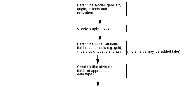
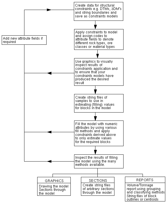
Flowchart for Simple Use of Block Modelling